“Airmass” redirects here. For the meteorology concept, see air mass. For solar energy applications, see air mass (solar energy).
In astronomy, air mass or airmass is a measure of the amount of air along the line of sight when observing a star or other celestial source from below Earth’s atmosphere (Green 1992). It is formulated as the integral of air density along the light ray.
As it penetrates the atmosphere, light is attenuated by scattering and absorption; the thicker atmosphere through which it passes, the greater the attenuation. Consequently, celestial bodies when nearer the horizon appear less bright than when nearer the zenith. This attenuation, known as atmospheric extinction, is described quantitatively by the Beer–Lambert law.
“Air mass” normally indicates relative air mass, the ratio of absolute air masses (as defined above) at oblique incidence relative to that at zenith. So, by definition, the relative air mass at the zenith is 1. Air mass increases as the angle between the source and the zenith increases, reaching a value of approximately 38 at the horizon. Air mass can be less than one at an elevation greater than sea level; however, most closed-form expressions for air mass do not include the effects of the observer’s elevation, so adjustment must usually be accomplished by other means.
Tables of air mass have been published by numerous authors, including Bemporad (1904), Allen (1973),[1] and Kasten & Young (1989).
Definition[edit]
The absolute air mass is defined as:

where 

In the vertical direction, the absolute air mass at zenith is:

So 
Finally, the relative air mass is:

Assuming air density is uniform allows removing it out of the integrals. The absolute air mass then simplifies to a product:

where 


In the corresponding simplified relative air mass, the average density cancels out in the fraction, leading to the ratio of path lengths:

Further simplifications are often made, assuming straight-line propagation (neglecting ray bending), as discussed below.
Calculation[edit]

Plots of air mass using various formulas
Background[edit]
The angle of a celestial body with the zenith is the zenith angle (in astronomy, commonly referred to as the zenith distance). A body’s angular position can also be given in terms of altitude, the angle above the geometric horizon; the altitude 


Atmospheric refraction causes light entering the atmosphere to follow an approximately circular path that is slightly longer than the geometric path. Air mass must take into account the longer path (Young 1994). Additionally, refraction causes a celestial body to appear higher above the horizon than it actually is; at the horizon, the difference between the true zenith angle and the apparent zenith angle is approximately 34 minutes of arc. Most air mass formulas are based on the apparent zenith angle, but some are based on the true zenith angle, so it is important to ensure that the correct value is used, especially near the horizon.[2]
Plane-parallel atmosphere[edit]
When the zenith angle is small to moderate, a good approximation is given by assuming a homogeneous plane-parallel atmosphere (i.e., one in which density is constant and Earth’s curvature is ignored). The air mass 

At a zenith angle of 60°, the air mass is approximately 2. However, because the Earth is not flat, this formula is only usable for zenith angles up to about 60° to 75°, depending on accuracy requirements. At greater zenith angles, the accuracy degrades rapidly, with 
Interpolative formulas[edit]
Many formulas have been developed to fit tabular values of air mass; one by Young & Irvine (1967) included a simple corrective term:
![{displaystyle X=sec ,z_{mathrm {t} },left[1-0.0012,(sec ^{2}z_{mathrm {t} }-1)right],,}](https://wikimedia.org/api/rest_v1/media/math/render/svg/c155681fae8813880954846c9e7d0c97173f5028)
where 
Hardie (1962) introduced a polynomial in 

which gives usable results for zenith angles of up to perhaps 85°. As with the previous formula, the calculated air mass reaches a maximum, and then approaches negative infinity at the horizon.
Rozenberg (1966) suggested

which gives reasonable results for high zenith angles, with a horizon air mass of 40.
Kasten & Young (1989) developed[3]

which gives reasonable results for zenith angles of up to 90°, with an air mass of approximately 38 at the horizon. Here the second
Young (1994) developed

in terms of the true zenith angle
Pickering (2002) developed

where 
Atmospheric models[edit]
Interpolative formulas attempt to provide a good fit to tabular values of air mass using minimal computational overhead. The tabular values, however, must be determined from measurements or atmospheric models that derive from geometrical and physical considerations of Earth and its atmosphere.
Nonrefracting spherical atmosphere[edit]

Atmospheric effects on optical transmission can be modelled as if the atmosphere is concentrated in approximately the lower 9 km.
If atmospheric refraction is ignored, it can be shown from simple geometrical considerations (Schoenberg 1929, 173) that the path


or alternatively,

where 
The relative air mass is then:

Homogeneous atmosphere[edit]
If the atmosphere is homogeneous (i.e., density is constant), the atmospheric height

where 


Taking 


The homogeneous spherical model slightly underestimates the rate of increase in air mass near the horizon; a reasonable overall fit to values determined from more rigorous models can be had by setting the air mass to match a value at a zenith angle less than 90°. The air mass equation can be rearranged to give

matching Bemporad’s value of 19.787 at
gives 

While a homogeneous atmosphere isn’t a physically realistic model, the approximation is reasonable as long as the scale height of the atmosphere is small compared to the radius of the planet. The model is usable (i.e., it does not diverge or go to zero) at all zenith angles, including those greater than 90° (see § Homogeneous spherical atmosphere with elevated observer). The model requires comparatively little computational overhead, and if high accuracy is not required, it gives reasonable results.[5]
However, for zenith angles less than 90°, a better fit to accepted values of air mass can be had with several
of the interpolative formulas.
Variable-density atmosphere[edit]
In a real atmosphere, density is not constant (it decreases with elevation above mean sea level. The absolute air mass for the geometrical light path discussed above, becomes, for a sea-level observer,

Isothermal atmosphere[edit]
Several basic models for density variation with elevation are commonly used. The simplest, an isothermal atmosphere, gives

where 


An approximate correction for refraction can be made by taking (Young 1974, p. 147)

where

Using a scale height of 8435 m, Earth’s mean radius of 6371 km, and including the correction for refraction,

Polytropic atmosphere[edit]
The assumption of constant temperature is simplistic; a more realistic model is the polytropic atmosphere, for which

where 

where 
Layered atmosphere[edit]
Earth’s atmosphere consists of multiple layers with different temperature and density characteristics; common atmospheric models include the International Standard Atmosphere and the US Standard Atmosphere. A good approximation for many purposes is a polytropic troposphere of 11 km height with a lapse rate of 6.5 K/km and an isothermal stratosphere of infinite height (Garfinkel 1967), which corresponds very closely to the first two layers of the International Standard Atmosphere. More layers can be used if greater accuracy is required.[6]
Refracting radially symmetrical atmosphere[edit]
When atmospheric refraction is considered, ray tracing becomes necessary (Kivalov 2007), and the absolute air mass integral becomes[7]

where 


Rearrangement and substitution into the absolute air mass integral gives

The quantity 

![{displaystyle sigma =int _{r_{mathrm {obs} }}^{r_{mathrm {atm} }}{frac {rho ,mathrm {d} r}{sqrt {1-left[1+2(n_{mathrm {obs} }-1)(1-{frac {rho }{rho _{mathrm {obs} }}})right]left({frac {r_{mathrm {obs} }}{r}}right)^{2}sin ^{2}z}}},.}](https://wikimedia.org/api/rest_v1/media/math/render/svg/a1c692080a9bf803d87372a5ac20830eb23345c8)
Homogeneous spherical atmosphere with elevated observer[edit]
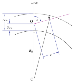
Air mass for elevated observer in homogeneous spherical atmosphere
In the figure at right, an observer at O is at an elevation

expanding the left- and right-hand sides, eliminating the common terms, and rearranging gives

Solving the quadratic for the path length s, factoring, and rearranging,

The negative sign of the radical gives a negative result, which is not physically meaningful. Using the positive sign, dividing by

With the substitutions 


When the observer’s elevation is zero, the air mass equation simplifies to

In the limit of grazing incidence, the absolute airmass equals the distance to the horizon. Furthermore, if the observer is elevated, the horizon zenith angle can be greater than 90°.

Maximum zenith angle for elevated observer in homogeneous spherical atmosphere
Nonuniform distribution of attenuating species[edit]
Atmospheric models that derive from hydrostatic considerations assume an atmosphere of constant composition and a single mechanism of extinction, which isn’t quite correct. There are three main sources of attenuation (Hayes & Latham 1975): Rayleigh scattering by air molecules, Mie scattering by aerosols, and molecular absorption (primarily by ozone). The relative contribution of each source varies with elevation above sea level, and the concentrations of aerosols and ozone cannot be derived simply from hydrostatic considerations.
Rigorously, when the extinction coefficient depends on elevation, it must be determined as part of the air mass integral, as described by Thomason, Herman & Reagan (1983). A compromise approach often is possible, however. Methods for separately calculating the extinction from each species using closed-form expressions are described in Schaefer (1993) and Schaefer (1998). The latter reference includes source code for a BASIC program to perform the calculations. Reasonably accurate calculation of extinction can sometimes be done by using one of the simple air mass formulas and separately determining extinction coefficients for each of the attenuating species (Green 1992, Pickering 2002).
Implications[edit]
Air mass and astronomy[edit]
![]()
In optical astronomy, the air mass provides an indication of the deterioration of the observed image, not only as regards direct effects of spectral absorption, scattering and reduced brightness, but also an aggregation of visual aberrations, e.g. resulting from atmospheric turbulence, collectively referred to as the quality of the “seeing”.[8] On bigger telescopes, such as the WHT (Wynne & Worswick 1988) and VLT (Avila, Rupprecht & Beckers 1997), the atmospheric dispersion can be so severe that it affects the pointing of the telescope to the target. In such cases an atmospheric dispersion compensator is used, which usually consists of two prisms.
The Greenwood frequency and Fried parameter, both relevant for adaptive optics, depend on the air mass above them (or more specifically, on the zenith angle).
In radio astronomy the air mass (which influences the optical path length) is not relevant. The lower layers of the atmosphere, modeled by the air mass, do not significantly impede radio waves, which are of much lower frequency than optical waves. Instead, some radio waves are affected by the ionosphere in the upper atmosphere. Newer aperture synthesis radio telescopes are especially affected by this as they “see” a much larger portion of the sky and thus the ionosphere. In fact, LOFAR needs to explicitly calibrate for these distorting effects (van der Tol & van der Veen 2007; de Vos, Gunst & Nijboer 2009), but on the other hand can also study the ionosphere by instead measuring these distortions (Thidé 2007).
Air mass and solar energy[edit]

Solar irradiance spectrum above atmosphere and at surface
In some fields, such as solar energy and photovoltaics, air mass is indicated by the acronym AM; additionally, the value of the air mass is often given by appending its value to AM, so that AM1 indicates an air mass of 1, AM2 indicates an air mass of 2, and so on. The region above Earth’s atmosphere, where there is no atmospheric attenuation of solar radiation, is considered to have “air mass zero” (AM0).
Atmospheric attenuation of solar radiation is not the same for all wavelengths; consequently, passage through the atmosphere not only reduces intensity but also alters the spectral irradiance. Photovoltaic modules are commonly rated using spectral irradiance for an air mass of 1.5 (AM1.5); tables of these standard spectra are given in ASTM G 173-03. The extraterrestrial spectral irradiance (i.e., that for AM0) is given in ASTM E 490-00a.[9]
For many solar energy applications when high accuracy near the horizon is not required, air mass is commonly determined using the simple secant formula described in the section Plane-parallel atmosphere.
See also[edit]
- Air mass (solar energy)
- Atmospheric extinction
- Beer–Lambert–Bouguer law
- Chapman function
- Computation of radiowave attenuation in the atmosphere
- Diffuse sky radiation
- Extinction coefficient
- Illuminance
- International Standard Atmosphere
- Irradiance
- Law of atmospheres
- Light diffusion
- Mie scattering
- Path loss
- Photovoltaic module
- Rayleigh scattering
- Solar irradiation
Notes[edit]
- ^ Allen’s air mass table was an abbreviated compilation of values from earlier sources, primarily Bemporad (1904).
- ^ At very high zenith angles, air mass is strongly dependent on local atmospheric conditions, including temperature, pressure, and especially the temperature gradient near the ground. In addition low-altitude extinction is strongly affected by the aerosol concentration and its vertical distribution. Many authors have cautioned that accurate calculation of air mass near the horizon is all but impossible.
- ^ The Kasten and Young formula was originally given in terms of altitude
as
in this article, it is given in terms of zenith angle for consistency with the other formulas.
- ^ Pickering (2002) uses Garfinkel (1967) as the reference for accuracy.
- ^ Although acknowledging that an isothermal or polytropic atmosphere would have been more realistic, Janiczek & DeYoung (1987) used the homogeneous spherical model in calculating illumination from the Sun and Moon, with the implication that the slightly reduced accuracy was more than offset by the considerable reduction in computational overhead.
- ^ The notes for Reed Meyer’s air mass calculator describe an atmospheric model using eight layers and using polynomials rather than simple linear relations for temperature lapse rates.
- ^ See Thomason, Herman & Reagan (1983) for a derivation of the integral for a refracting atmosphere.
- ^ Observing tips: air mass and differential refraction retrieved 15 May 2011.
- ^ ASTM E 490-00a was reapproved without change in 2006.

References[edit]
- Allen, C. W. (1973). Astrophysical Quantities (3rd ed.). London: Athlone, 125.: Athlone Press. ISBN 0-485-11150-0. OCLC 952445.
{{cite book}}: CS1 maint: location (link) - ASTM E 490-00a (R2006). 2000. Standard Solar Constant and Zero Air Mass Solar Spectral Irradiance Tables. West Conshohocken, PA: ASTM. Available for purchase from ASTM.Optical Telescopes of Today and Tomorrow
- ASTM G 173-03. 2003. Standard Tables for Reference Solar Spectral Irradiances: Direct Normal and Hemispherical on 37° Tilted Surface. West Conshohocken, PA: ASTM. Available for purchase from ASTM.
- Avila, Gerardo; Rupprecht, Gero; Beckers, J. M. (1997). Arne L. Ardeberg (ed.). “Atmospheric dispersion correction for the FORS Focal Reducers at the ESO VLT”. Optical Telescopes of Today and Tomorrow. Proceedings of SPIE. 2871 Optical Telescopes of Today and Tomorrow: 1135–1143. Bibcode:1997SPIE.2871.1135A. doi:10.1117/12.269000. S2CID 120965966.
- Bemporad, A. 1904. Zur Theorie der Extinktion des Lichtes in der Erdatmosphäre. Mitteilungen der Grossh. Sternwarte zu Heidelberg Nr. 4, 1–78.
- Garfinkel, Boris (1967). “Astronomical Refraction in a Polytropic Atmosphere”. The Astronomical Journal. 72: 235–254. Bibcode:1967AJ…..72..235G. doi:10.1086/110225.
- Green, Daniel W. E. 1992. Magnitude Corrections for Atmospheric Extinction. International Comet Quarterly 14, July 1992, 55–59.
- Hardie, R. H. 1962. In Astronomical Techniques. Hiltner, W. A., ed. Chicago: University of Chicago Press, 184–. LCCN 62009113. Bibcode 1962aste.book…..H.
- Kivalov, Sergey N. (2007). “Improved ray tracing air mass numbers model”. Applied Optics. 46 (29): 7091–8. Bibcode:2007ApOpt..46.7091K. doi:10.1364/AO.46.007091. ISSN 0003-6935. PMID 17932515.
- Hayes, D. S.; Latham, D. W. (1975). “A Rediscussion of the Atmospheric Extinction and the Absolute Spectral-Energy Distribution of Vega”. The Astrophysical Journal. 197: 593–601. Bibcode:1975ApJ…197..593H. doi:10.1086/153548. ISSN 0004-637X.
- Janiczek, P. M., and J. A. DeYoung. 1987. Computer Programs for Sun and Moon Illuminance with Contingent Tables and Diagrams, United States Naval Observatory Circular No. 171. Washington, D.C.: United States Naval Observatory. Bibcode 1987USNOC.171…..J.
- Kasten, F.; Young, A. T. (1989). “Revised optical air mass tables and approximation formula”. Applied Optics. 28 (22): 4735–4738. Bibcode:1989ApOpt..28.4735K. doi:10.1364/AO.28.004735. PMID 20555942.
- Pickering, K. A. (2002). “The Southern Limits of the Ancient Star Catalog” (PDF). DIO. 12 (1): 20–39.
- Rozenberg, Grzegorz V. (1966). Twilight: A Study in Atmospheric Optics. New York: Plenum Press. ISBN 978-1-4899-6353-6. LCCN 65011345. OCLC 1066196615.
- Schaefer, Bradley E. (1993). “Astronomy and the Limits of Vision”. Vistas in Astronomy. 36: 311–361. Bibcode:1993VA…..36..311S. doi:10.1016/0083-6656(93)90113-X.
- Schaefer, B. E. 1998. To the Visual Limits: How deep can you see?. Sky & Telescope, May 1998, 57–60.
- Schoenberg, E. 1929. Theoretische Photometrie, Über die Extinktion des Lichtes in der Erdatmosphäre. In Handbuch der Astrophysik. Band II, erste Hälfte. Berlin: Springer.
- Thidé, Bo (2007-12-01). “Nonlinear physics of the ionosphere and LOIS/LOFAR”. Plasma Physics and Controlled Fusion. 49 (12B): B103–B107. Bibcode:2007PPCF…49..103T. doi:10.1088/0741-3335/49/12B/S09. ISSN 0741-3335.
- Thomason, L. W.; Herman, B. M.; Reagan, J. A. (1983-07-01). “The Effect of Atmospheric Attenuators with Structured Vertical Distributions on Air Mass Determinations and Langley Plot Analyses”. Journal of the Atmospheric Sciences. 40 (7): 1851–1854. Bibcode:1983JAtS…40.1851T. doi:10.1175/1520-0469(1983)040<1851:TEOAAW>2.0.CO;2. ISSN 0022-4928.
- van der Tol, Sebastiaan; van der Veen, Alle-Jan (2007). “Ionospheric Calibration for the LOFAR Radio Telescope”. 2007 International Symposium on Signals, Circuits and Systems. 2: 1–4. doi:10.1109/ISSCS.2007.4292761.
- de Vos, M.; Gunst, A. W.; Nijboer, R. (2009). “The LOFAR Telescope: System Architecture and Signal Processing” (PDF). Proceedings of the IEEE. 97 (8): 1431–1437. Bibcode:2009IEEEP..97.1431D. doi:10.1109/JPROC.2009.2020509. ISSN 0018-9219.
- Wynne, C. G.; Worswick, S. P. (1988-02-01). “Atmospheric dispersion at prime focus”. Monthly Notices of the Royal Astronomical Society. 230 (3): 457–471. Bibcode:1988MNRAS.230..457W. doi:10.1093/mnras/230.3.457. ISSN 0035-8711.
- Young, A. T. 1974. Atmospheric Extinction. Ch. 3.1 in Methods of Experimental Physics, Vol. 12 Astrophysics, Part A: Optical and Infrared. ed. N. Carleton. New York: Academic Press. ISBN 0-12-474912-1.
- Young, Andrew T. (1994-02-20). “Air Mass and Refraction”. Applied Optics. 33 (6): 1108. Bibcode:1994ApOpt..33.1108Y. doi:10.1364/AO.33.001108. ISSN 0003-6935.
- Young, Andrew T.; Irvine, William M. (1967). “Multicolor photoelectric photometry of the brighter planets. I. Program and Procedure”. The Astronomical Journal. 72: 945–950. Bibcode:1967AJ…..72..945Y. doi:10.1086/110366.
External links[edit]
- Reed Meyer’s downloadable airmass calculator, written in C (notes in the source code describe the theory in detail)
- NASA Astrophysics Data System A source for electronic copies of some of the references.
Как найти массу воздуха
Воздух – это естественная смесь газов, состоящая, большей частью, из азота и кислорода. Масса воздуха в единице объема может меняться, если меняются пропорции составляющих его компонентов, а также при изменении температуры. Массу воздуха можно найти, зная объем, который он занимает, или количество вещества (количество частиц).
Вам понадобится
- плотность воздуха, молярная масса воздуха, количество воздуха, объем, занимаемый воздухом
Инструкция
Пусть нам известен объем V, который занимает воздух. Тогда по известной формуле m = p*V, где – p – плотность воздуха, мы можем найти массу воздуха в этом объеме.
Плотность воздуха зависит от его температуры. Плотность сухого воздуха вычисляется через уравнение Клапейрона для идеального газа по формуле: p = P/(R*T), где P – абсолютное давление, T – абсолютная температура в Кельвинах, а R – удельная газовая постоянная для сухого воздуха (R = 287,058 Дж/(кг*К)).
На уровне моря при температуре 0оС плотность воздуха равна 1,2920 кг/(м^3).
Если известно количество воздуха, то его массу можно найти по формуле: m = M*V, где V – количество вещества в молях, а M – молярная масса воздуха. Средняя относительная молярная масса воздуха равна 28,98 г/моль. Таким образом, подставив ее в эту формулу, вы получите массу воздуха в граммах.
Источники:
- Физические свойства воздуха
Войти на сайт
или
Забыли пароль?
Еще не зарегистрированы?
This site is protected by reCAPTCHA and the Google Privacy Policy and Terms of Service apply.
Количество воздуха, видимое в астрономических наблюдениях
В астрономии, воздушная масса или воздушная масса – это «количество воздуха, которое просматривается» (зеленый 1992), когда видит звезду или другую небесный источник снизу атмосфера Земли. Он формулируется как интеграл от плотности воздуха вдоль светового луча .
. Когда он проникает в атмосферу, свет ослабляется за счет рассеяния и поглощение ; чем плотнее атмосфера, через которую он проходит, тем больше затухание . Следовательно, небесные тела, когда они приближаются к горизонту, кажутся менее яркими, чем когда они ближе к зениту. Это затухание, известное как атмосферное ослабление, количественно описывается законом Бера – Ламберта.
«Воздушная масса» обычно указывает относительную воздушную массу, отношение абсолютных воздушных масс (как определено выше) при наклонном падении относительно угла падения в зените. Итак, по определению, относительная масса воздуха в зените равна 1. Масса воздуха увеличивается по мере увеличения угла между источником и зенитом, достигая значения примерно 38 на горизонте. Воздушная масса может быть меньше единицы на высоте выше уровня моря ; однако большинство выражений в замкнутой форме для воздушной массы не включают эффекты возвышения наблюдателя, поэтому корректировка обычно должна выполняться другими способами.
Таблицы воздушных масс были опубликованы многими авторами, включая Бемпорада (1904),, Аллена (1976), и Kasten and Young (1989)..
Содержание
- 1 Определение
- 2 Расчет
- 2.1 Предпосылки
- 2.2 Плоскопараллельная атмосфера
- 2.3 Интерполяционные формулы
- 2.4 Атмосферные модели
- 2.4.1 Неотражающая сферическая атмосфера
- 2.4.2 Однородная атмосфера
- 2.4.3 Атмосфера переменной плотности
- 2.4.4 Изотермическая атмосфера
- 2.4.5 Политропная атмосфера
- 2.4.6 Слоистая атмосфера
- 2.4.7 преломляющая радиально-симметричная атмосфера
- 2.4.8 Однородная сферическая атмосфера с приподнятым наблюдателем
- 2.5 Неравномерное распределение ослабляющих частиц
- 3 Последствия
- 3.1 Воздушная масса и астрономия
- 3.2 Воздушная масса и солнечная энергия
- 4 См. Также
- 5 Примечания
- 6 Ссылки
- 7 Внешние ссылки
Определение
Абсолютная воздушная масса определяется как:
- σ = ∫ ρ ds. { displaystyle sigma = int rho , mathrm {d} s ,.}
, где ρ { displaystyle rho}
В вертикальном направлении абсолютная масса воздуха в зените составляет:
- σ дзен = ∫ ρ dz { displaystyle sigma _ { mathrm {zen}} = int rho , mathrm {d} z}
Итак σ zen { displaystyle sigma _ { mathrm {zen}}}
Наконец, относительная масса воздуха:
- X = σ σ zen { displaystyle X = { frac { sigma} { sigma _ { mathrm {zen}}}}}
. Предполагая, что плотность воздуха однородна, можно исключить ее из интегралов. Абсолютная воздушная масса затем упрощается до произведения:
- σ = ρ ¯ s { displaystyle sigma = { bar { rho}} s}
где ρ ¯ = c o n s t. { displaystyle { bar { rho}} = mathrm {const.}}
- s = ∫ ds { displaystyle s = int , mathrm {d} s}
- szen = ∫ dz { displaystyle s _ { mathrm {zen}} = int , mathrm {d} z}


В соответствующей упрощенной относительной воздушной массе средняя плотность сокращается в долях, что приводит к соотношению длин пути:
- X = sszen. { displaystyle X = { frac {s} {s _ { mathrm {zen}}}} ,.}
Часто делаются дальнейшие упрощения, предполагая прямолинейное распространение (без учета изгиба лучей), как описано ниже.
Расчет
 Графики массы воздуха с использованием различных формул.
Предпосылки
Угол зенита небесного тела равен зенитному углу (в астрономии, обычно называемое зенитным расстоянием ). Угловое положение тела также может быть задано в виде высоты, угла над геометрическим горизонтом; высота h { displaystyle h}
- h = 90 ∘ – z. { displaystyle h = 90 ^ { circ} -z ,.}
Атмосферная рефракция заставляет свет, входящий в атмосферу, следовать приблизительно по круговой траектории, которая немного длиннее геометрической траектории. Воздушная масса должна учитывать более длинный путь (Young 1994). Вдобавок рефракция заставляет небесное тело казаться выше горизонта, чем оно есть на самом деле; на горизонте разница между истинным зенитным углом и видимым зенитным углом составляет приблизительно 34 угловые минуты. Большинство формул воздушных масс основаны на кажущемся зенитном угле, но некоторые основаны на истинном зенитном угле, поэтому важно убедиться, что используется правильное значение, особенно вблизи горизонта.
Плоскопараллельная атмосфера
Когда зенитный угол от малого до умеренного, хорошее приближение дается в предположении однородной плоскопараллельной атмосферы (т. Е. Такой, в которой плотность постоянна, а кривизна Земли не учитывается). Тогда воздушная масса X { displaystyle X}
- X = sec z. { displaystyle X = sec , z ,.}
При зенитном угле 60 ° масса воздуха равна примерно 2. Однако, поскольку Земля не плоская, эта формула имеет вид может использоваться только для зенитных углов примерно от 60 ° до 75 °, в зависимости от требований к точности. При больших зенитных углах точность быстро ухудшается, и X = sec z { displaystyle X = sec , z}
Интерполяционные формулы
Многие формулы были разработаны для соответствия табличным значениям воздушной массы; автор Янга и Ирвина (1967) включил простой корректирующий член:
- X = sec zt [1 – 0,0012 (sec 2 zt – 1)], { displaystyle X = sec , z _ { mathrm {t}} , left [1-0.0012 , ( sec ^ {2} z _ { mathrm {t}} -1) right] ,,}
где zt { displaystyle z _ { mathrm {t}}}
Харди (1962) ввел многочлен в сек z – 1 { displaystyle sec , z-1}
- X = sec z – 0,0018167 (сек z – 1) – 0,002875 ( сек z – 1) 2 – 0,0008083 (сек z – 1) 3 { displaystyle X = sec , z , – , 0,0018167 , ( sec , z , – , 1) , – , 0.002875 , ( sec , z , – , 1) ^ {2} , – , 0.0008083 , ( sec , z , – , 1) ^ {3} ,}

, что дает полезные результаты для зенитных углов, возможно, до 85 °. Как и в предыдущей формуле, расчетная воздушная масса достигает максимума, а затем приближается к отрицательной бесконечности на горизонте.
Розенберг (1966) предложил
- X = (cos z + 0,025 e – 11 cos z) – 1, { displaystyle X = left ( cos , z + 0,025e ^ {- 11 cos , z} right) ^ {- 1} ,,}
, который дает разумные результаты для больших зенитных углов с горизонтальной воздушной массой 40.
Kasten and Young (1989) развернутое
- X = 1 cos z + 0.50572 (6.07995 ∘ + 90 ∘ – z) – 1.6364, { displaystyle X = { frac {1} { cos , z + 0.50572 , (6.07995 ^ { circ } +90 ^ { circ} -z) ^ {- 1.6364}}} ,,}
, что дает разумные результаты для зенитных углов до 90 ° с воздушной массой около 38 на горизонте. Здесь второй член z { displaystyle z}
Янг (1994) разработал
- X = 1,002432 cos 2 zt + 0,148386 cos zt + 0,0096467 cos 3 zt + 0,149864 cos 2 zt + 0,0102963 cos zt + 0,000303978 { displaystyle X = { гидроразрыв {1.002432 , cos ^ {2} z _ { mathrm {t}} +0.148386 , cos , z _ { mathrm {t}} +0.0096467} { cos ^ {3} z _ { mathrm { t}} +0.149864 , cos ^ {2} z _ { mathrm {t}} +0.0102963 , cos , z _ { mathrm {t}} +0.000303978}} ,}
в терминах истинный зенитный угол zt { displaystyle z _ { mathrm {t}}}
Пикеринг (2002) разработал
- X = 1 грех (h + 244 / (165 + 47 h 1.1)), { displaystyle X = { frac {1} { sin (h + { 244} / (165 + 47h ^ {1.1}))}} ,,}
где h { displaystyle h}
Атмосферные модели
Интерполяционные формулы пытаются обеспечить хорошее соответствие табличным значениям воздушной массы с минимальными вычислительными затратами. Табличные значения, однако, должны определяться на основе измерений или моделей атмосферы, которые вытекают из геометрических и физических соображений, касающихся Земли и ее атмосферы.
Неотражающая сферическая атмосфера
Атмосферные эффекты на оптическое пропускание могут быть смоделированы так, как если бы атмосфера концентрировалась приблизительно в нижних 9 км.
Если атмосферное преломление игнорировать, оно может из простых геометрических соображений (Schoenberg 1929, 173) показать, что путь s { displaystyle s}
- s = RE 2 соз 2 z + 2 RE yatm + yatm 2 – RE cos z { displaystyle s = { sqrt {R _ { mathrm {E}} ^ {2} cos ^ {2} z + 2R _ { mathrm {E }} y _ { mathrm {atm}} + y _ { mathrm {atm}} ^ {2}}} – R _ { mathrm {E}} cos , z ,}
или, альтернативно,
- s = (RE + yatm) 2 – RE 2 грех 2 Z – RE cos z { displaystyle s = { sqrt { left (R _ { mathrm {E}} + y _ { mathrm {atm}} справа) ^ {2} -R _ { mathrm {E}} ^ {2} sin ^ {2} z}} – R _ { mathrm {E}} cos , z ,}
где R E { displaystyle R _ { mathrm {E}}}
Тогда относительная масса воздуха равна:
- X = s y a t m = R E y a t m cos 2 z + 2 y a t m R E + (y a t m R E) 2 – R E y a t m cos z. { displaystyle X = { frac {s} {y _ { mathrm {atm}}}} = { frac {R _ { mathrm {E}}} {y _ { mathrm {atm}}}} { sqrt { cos ^ {2} z + 2 { frac {y _ { mathrm {atm}}} {R _ { mathrm {E}}}} + left ({ frac {y _ { mathrm {atm}}) } {R _ { mathrm {E}}}} right) ^ {2}}} – { frac {R _ { mathrm {E}}} {y _ { mathrm {atm}}}} cos , z ,.}
Однородная атмосфера
Если атмосфера однородная (т. е. плотность постоянна), высота атмосферы yatm { displaystyle y _ { mathrm {atm}}}
- yatm = k T 0 mg, { displaystyle y _ { mathrm {atm}} = { frac {kT_ {0}} {mg}} ,,}
где k { displaystyle k}
Принимая T 0 { displaystyle T_ {0}}
- X h o r i z = 1 + 2 R E y a t m ≈ 38,87. { displaystyle X _ { mathrm {horizon}} = { sqrt {1 + 2 { frac {R _ { mathrm {E}}} {y _ { mathrm {atm}}}}}} приблизительно 38,87 ,.}
Однородная сферическая модель немного занижает скорость увеличения воздушной массы около горизонта; разумное полное соответствие значениям, определенным на основе более строгих моделей, может быть достигнуто путем настройки воздушной массы, соответствующей значению при зенитном угле менее 90 °. Уравнение воздушных масс может быть преобразовано в
- R E y a t m = X 2 – 1 2 (1 – X cos z); { displaystyle { frac {R _ { mathrm {E}}} {y _ { mathrm {atm}}}} = { frac {X ^ {2} -1} {2 left (1-X cos z right)}} ,;}
соответствие значению Бемпорада 19,787 при z { displaystyle z}
Хотя однородная атмосфера не является физически реалистичной моделью, приближение разумно, если масштабная высота атмосферы мала по сравнению с радиусом планеты. Модель может использоваться (т.е. она не расходится и не стремится к нулю) при всех зенитных углах, включая углы, превышающие 90 ° (см. Однородная сферическая атмосфера с приподнятым наблюдателем ниже). Модель требует сравнительно небольших вычислительных затрат и, если не требуется высокой точности, дает разумные результаты. Однако для зенитных углов менее 90 ° большее соответствие принятым значениям воздушной массы может быть получено с помощью нескольких интерполяционных формул.
Атмосфера переменной плотности
В реальной атмосфере плотность непостоянна (она уменьшается с высотой выше среднего уровня моря. Абсолютная воздушная масса для геометрического светового пути обсуждалось выше, становится для наблюдателя на уровне моря
- σ = ∫ 0 yatm ρ (RE + y) dy RE 2 cos 2 z + 2 RE y + y 2. { displaystyle sigma = int _ {0} ^ {y _ { mathrm {atm}}} { frac { rho , left (R _ { mathrm {E}} + y right) mathrm {d} y} { sqrt {R_ { mathrm {E}} ^ {2} cos ^ {2} z + 2R _ { mathrm {E}} y + y ^ {2}}}} ,.}
Изотермическая атмосфера
Обычно используется несколько основных моделей изменения плотности с высотой. Простейшая, изотермическая атмосфера, дает
- ρ = ρ 0 e – y / H, { displaystyle rho = rho _ {0} e ^ {- y / H} ,,}
где ρ 0 { displaystyle rho _ {0}}
- X ≈ π R 2 H exp (R cos 2 z 2 H) e r f c (R cos 2 z 2 H). { displaystyle X приблизительно { sqrt { frac { pi R} {2H}}} exp { left ({ frac {R cos ^ {2} z} {2H}} right)} , mathrm {erfc} left ({ sqrt { frac {R cos ^ {2} z} {2H}}} right) ,.}
Приблизительную поправку на рефракцию можно сделать, взяв (Янг 1974, 147)
- R = 7/6 RE, { displaystyle R = 7/6 , R _ { mathrm {E}} ,,}
где RE { displaystyle R _ { mathrm {E}}}
- X h o r i z ≈ π R 2 H. { displaystyle X _ { mathrm {horizon}} приблизительно { sqrt { frac { pi R} {2H}}} ,.}
Используя масштаб высоты 8435 м, средний радиус Земли 6371 км, включая поправку на рефракцию,
- X горизонт ≈ 37.20. { displaystyle X _ { mathrm {Horiz}} приблизительно 37.20 ,.}
Политропическая атмосфера
Предположение о постоянной температуре является упрощенным; более реалистичной моделью является политропная атмосфера, для которой
- T = T 0 – α y, { displaystyle T = T_ {0} – alpha y ,,}
где T 0 { displaystyle T_ {0}}
- ρ = ρ 0 (1 – α T 0 y) 1 / (κ – 1), { displaystyle rho = rho _ {0} left (1 – { гидроразрыв { alpha} {T}} _ {0} y right) ^ {1 / ( kappa -1)} ,,}
где κ { displaystyle kappa}
Слоистая атмосфера
Атмосфера Земли состоит из нескольких слоев с различными температурными и плотностными характеристиками; общие модели атмосферы включают международную стандартную атмосферу и стандартную атмосферу США. Хорошим приближением для многих целей является политропическая тропосфера высотой 11 км с градиентом 6,5 К / км и изотермическая стратосфера бесконечной высоты (Гарфинкель 1967), что очень близко соответствует первым двум слоям Международной стандартной атмосферы. Если требуется большая точность, можно использовать больше слоев.
Преломляющая радиально-симметричная атмосфера
Когда учитывается атмосферная рефракция, трассировка лучей становится необходимой, и абсолютный интеграл воздушных масс становится
- σ = ∫ robsratm ρ dr 1 – (nobsnrobsr) 2 sin 2 z { displaystyle sigma = int _ {r _ { mathrm {obs}}} ^ {r _ { mathrm {atm}}} { frac { rho , mathrm {d} r} { sqrt {1- left ({ frac {n _ { mathrm {obs}}} {n}} { frac {r _ { mathrm { obs}}} {r}} right) ^ {2} sin ^ {2} z}}} ,}
где nobs { displaystyle n _ { mathrm {obs}}}
- n – 1 n o b s – 1 = ρ ρ o b s. { displaystyle { frac {n-1} {n _ { mathrm {obs}} -1}} = { frac { rho} { rho _ { mathrm {obs}}}} ,.}
Перестановка и подстановка в абсолютный интеграл воздушных масс дает
- σ = ∫ robsratm ρ dr 1 – (nobs 1 + (nobs – 1) ρ / ρ obs) 2 (robsr) 2 sin 2 z. { displaystyle sigma = int _ {r _ { mathrm {obs}}} ^ {r _ { mathrm {atm}}} { frac { rho , mathrm {d} r} { sqrt {1 – left ({ frac {n _ { mathrm {obs}}} {1+ (n _ { mathrm {obs}} -1) rho / rho _ { mathrm {obs}}}} right) ^ {2} left ({ frac {r _ { mathrm {obs}}} {r}} right) ^ {2} sin ^ {2} z}}} ,.}
Количество nobs – 1 { displaystyle n _ { mathrm {obs}} -1}
- σ = ∫ robsratm ρ dr 1 – [1 + 2 (nobs – 1) (1 – ρ ρ obs)] (robsr) 2 sin 2 z. { displaystyle sigma = int _ {r _ { mathrm {obs}}} ^ {r _ { mathrm {atm}}} { frac { rho , mathrm {d} r} { sqrt {1 – left [1 + 2 (n _ { mathrm {obs}} -1) (1 – { frac { rho} { rho _ { mathrm {obs}}}}) right] left ({ frac {r _ { mathrm {obs}}} {r}} right) ^ {2} sin ^ {2} z}}} ,.}
Однородная сферическая атмосфера с приподнятым наблюдателем
Воздух масса для наблюдателя, находящегося на возвышении в однородной сферической атмосфере
На рисунке справа наблюдатель в точке O находится на высоте yobs { displaystyle y _ { mathrm {obs}}}
- (RE + yatm) 2 = s 2 + (RE + yobs) 2-2 (RE + yobs) s cos (180 ∘ – z) знак равно s 2 + (RE + yobs) 2 + 2 (RE + yobs) s cos z { displaystyle { begin {align} left (R_ {E} + y_ {atm} right) ^ {2} = s ^ {2} + left (R_ {E} + y_ {obs} right) ^ {2} -2 left (R_ {E} + y_ {obs} right) s cos left (180 ^ { circ} -z right) \ = s ^ {2} + left (R_ {E} + y_ {obs} right) ^ {2} +2 left (R_ {E} + y_ {obs} right) s cos z end {align}}}
расширение левой и правой частей, удаление общих терминов и перестановка дает
- s 2 + 2 (RE + y obs) s cos z – 2 RE y atm – y atm 2 + 2 RE y obs + y obs 2 = 0. { displaystyle {{s} ^ {2}} + 2 left ({{R} _ { text {E}}} + {{y} _ { text {obs}}} right) s cos z-2 {{R} _ { text {E}}} {{y} _ { text {atm}}} – y _ { text {atm}} ^ {2} +2 {{R} _ { text {E}}} {{y} _ { text {obs}}} + y _ { text {obs}} ^ {2} = 0 ,.}

Решение квадратичного уравнения для длины пути s, факторизация и преобразование,
- s = ± (RE + y obs) 2 cos 2 z + 2 RE (y atm – y obs) + y atm 2 – y obs 2 – (RE + y obs) cos z. { displaystyle s = pm { sqrt {{{ left ({{R} _ { text {E}}} + {{y} _ { text {obs}}} right)} ^ {2 }} {{ cos} ^ {2}} z + 2 {{R} _ { text {E}}} left ({{y} _ { text {atm}}} – {{y} _ { text {obs}} right) + y _ { text {atm}} ^ {2} -y _ { text {obs}} ^ {2}}} – ({{R} _ { text { E}}} + {{y} _ { text {obs}}}) cos z ,.}

Отрицательный знак радикала дает отрицательный результат, который не имеет физического смысла. Используя положительный знак, разделив на yatm { displaystyle y _ { mathrm {atm}}}
- X = (RE + y obs y atm) 2 cos 2 z + 2 RE y atm 2 (y atm – y obs) – (y obs y atm) 2 + 1 – RE + y obs y atm cos z. { displaystyle X = { sqrt {{{ left ({ frac {{{R} _ { text {E}}} + {{y} _ { text {obs}}}} {{y}) _ { text {atm}}}} right)} ^ {2}} {{ cos} ^ {2}} z + { frac {2 {{R} _ { text {E}}}} { y _ { text {atm}} ^ {2}}} left ({{y} _ { text {atm}}} – {{y} _ { text {obs}}} right) – {{ left ({ frac {{y} _ { text {obs}}} {{y} _ { text {atm}}}} right)} ^ {2}} + 1}} – { frac {{{R} _ { text {E}}} + {{y} _ { text {obs}}}} {{y} _ { text {atm}}}} cos z ,.}

С заменами r ^ = RE / yatm { displaystyle { hat {r}} = R _ { mathrm {E}} / y _ { mathrm {atm}}}
- X = (r ^ + y ^) 2 cos 2 z + 2 r ^ (1 – y ^) – y ^ 2 + 1 – (r ^ + y ^) cos z. { displaystyle X = { sqrt {{{({ hat {r}} + { hat {y}})} ^ {2}} {{ cos} ^ {2}} z + 2 { hat {r}} (1 – { hat {y}}) – { hat {y}} ^ {2} +1}} ; – ; ({ hat {r}} + { hat {y }}) cos z ,.}

Когда угол места наблюдателя равен нулю, уравнение воздушных масс упрощается до
- X = (RE y atm) 2 cos 2 z + 2 RE y atm + 1 – RE y атм cos z. { displaystyle X = { sqrt {{{ left ({ frac {{R} _ { text {E}}} {{y} _ { text {atm}}}} right)} ^ { 2}} {{ cos} ^ {2}} z + { frac {2 {{R} _ { text {E}}}} {{y} _ { text {atm}}}} + 1} } – { frac {{R} _ { text {E}}} {{y} _ { text {atm}}}} cos z ,.}

В пределе выпаса Абсолютная воздушная масса равна расстоянию до горизонта. Кроме того, если наблюдатель находится на высоте, зенитный угол горизонта может быть больше 90 °.
Максимальный зенитный угол для наблюдателя, находящегося на возвышении в однородной сферической атмосфере
Неравномерное распределение ослабляющих частиц
Атмосферные модели, основанные на гидростатических соображениях, предполагают постоянный состав атмосферы и единый механизм вымирания, который не является т совершенно правильно. Существует три основных источника ослабления (Hayes and Latham 1975): рэлеевское рассеяние на молекулах воздуха, рассеяние Ми на аэрозолях и молекулярное поглощение (в основном озоном ). Относительный вклад каждого источника изменяется в зависимости от высоты над уровнем моря, и концентрации аэрозолей и озона не могут быть получены просто из гидростатических соображений.
Строго говоря, когда коэффициент ослабления зависит от высоты, он должен определяться как часть интеграла воздушных масс, как описано Томасоном, Германом и Рейганом (1983). Однако зачастую возможен компромиссный подход. Методы отдельного расчета вымирания от каждого вида с использованием выражений в закрытой форме описаны в Schaefer (1993) и Schaefer (1998). Последняя ссылка включает исходный код для программы BASIC для выполнения вычислений. Достаточно точный расчет вымирания иногда может быть выполнен с использованием одной из простых формул воздушных масс и отдельного определения коэффициентов экстинкции для каждого из ослабляющих видов (Green 1992, Pickering 2002).
Значение
Воздушная масса и астрономия
![]() Пропускание атмосферы в электромагнитном спектре.
Пропускание атмосферы в электромагнитном спектре.
В оптической астрономии воздушная масса служит индикатором ухудшение наблюдаемого изображения не только в отношении прямых эффектов спектрального поглощения, рассеяния и пониженной яркости, но также и совокупность визуальных аберраций, например в результате атмосферной турбулентности, в совокупности называемой качеством «видения ». На больших телескопах, таких как WHT (Wynne and Warsick 1988) и VLT (Avila, Rupprecht, and Becker 1997), атмосферное рассеяние может быть настолько сильным, что влияет на наведение телескопа на цель. В таких случаях используется компенсатор атмосферной дисперсии, который обычно состоит из двух призм.
Частота Гринвуда и параметр Фрида, оба значимые для адаптивной оптики, зависят от воздушной массы над ними (или, более конкретно, от зенитный угол ).
В радиоастрономии воздушная масса (которая влияет на длину оптического пути) не имеет значения. Нижние слои атмосферы, моделируемые воздушной массой, не сильно препятствуют радиоволнам, которые имеют гораздо более низкую частоту, чем оптические волны. Вместо этого на некоторые радиоволны влияет ионосфера в верхних слоях атмосферы. Это особенно влияет на более новые радиотелескопы с синтезом апертуры , поскольку они «видят» гораздо большую часть неба и, следовательно, ионосферу. Фактически, LOFAR необходимо явно откалибровать для этих искажающих эффектов (van der Tol and van der Veen 2007 ; de Vos, Gunst, and Nijboer 2009), но, с другой стороны, можно также изучать ионосферу, вместо этого измеряя эти искажения (Thidé 2007).
Воздушная масса и солнечная энергия
Спектр солнечного излучения над атмосферой и у поверхности
В некоторых областях, таких как солнечная энергия и фотогальваника, воздушные массы обозначается аббревиатурой AM; Кроме того, значение воздушной массы часто задается путем добавления ее значения к AM, так что AM1 указывает на массу воздуха 1, AM2 указывает на массу воздуха 2 и так далее. Область над атмосферой Земли, где нет атмосферного ослабления солнечного излучения, считается имеющей «нулевую массу воздуха » (AM0).
Атмосферное ослабление солнечного излучения не одинаково для всех длин волн; следовательно, прохождение через атмосферу не только снижает интенсивность, но также изменяет спектральную освещенность. Фотоэлектрические модули обычно оцениваются с использованием спектральной энергетической освещенности для воздушной массы 1,5 (AM1,5); Таблицы этих стандартных спектров приведены в ASTM G 173-03. Спектральная энергетическая освещенность внеземных источников (т. Е. Для AM0) приведена в ASTM E 490-00a.
. Для многих приложений солнечной энергии, когда не требуется высокая точность вблизи горизонта, воздушная масса обычно определяется с использованием простой формулы секущей описано в разделе Плоскопараллельная атмосфера.
См. также
- Воздушная масса (солнечная энергия)
- Атмосферное вымирание
- Закон Бера – Ламберта – Бугера
- Рассеянное излучение неба
- Коэффициент ослабления
- Освещенность
- Международная стандартная атмосфера
- Излучение
- Закон атмосфер
- Рассеивание света
- Рассеяние Ми
- Потери на пути
- Фотоэлектрический модуль
- Рэлеевское рассеяние
- Солнечное излучение
Примечания
Ссылки
- Allen, CW 1976. Astrophysical Quantities, 3-е изд. 1973, перепечатано с исправлениями, 1976. Лондон: Athlone, 125. ISBN 0-485-11150-0 .
- ASTM E 490-00a (R2006). 2000. Таблицы стандартной солнечной постоянной и спектральной освещенности с нулевой массой воздуха. Вест Коншохокен, Пенсильвания: ASTM. Доступно для покупки в ASTM. Оптические телескопы сегодня и завтра
- ASTM G 173-03. 2003. Стандартные таблицы для эталонной солнечной спектральной освещенности: прямая нормальная и полусферическая на поверхности с наклоном 37 °. Вест Коншохокен, Пенсильвания: ASTM. Доступно для покупки в ASTM.
- Авила, Херардо; Рупрехт, Геро; Бекерс, Дж. М. (1997). Арне Л. Ардеберг (ред.). «Поправка атмосферной дисперсии для фокусных редукторов FORS в ESO VLT». Оптические телескопы сегодня и завтра. Труды SPIE. 2871 Оптические телескопы сегодня и завтра: 1135–1143. Bibcode : 1997SPIE.2871.1135A. doi : 10.1117 / 12.269000.
- Бемпорад, A. 1904. Zur Theorie der Extinktion des Lichtes in der Erdatmosphäre. Mitteilungen der Grossh. Sternwarte zu Heidelberg Nr. 4, 1–78.
- Гарфинкель Б. 1967. Астрономическая рефракция в политропной атмосфере. Астрономический журнал 72: 235–254. doi : 10.1086 / 110225. Bibcode 1967AJ….. 72..235G.
- Грин, Дэниел У. Э. 1992. Поправки на величину атмосферного поглощения. International Comet Quarterly, 14 июля 1992 г., стр. 55–59.
- Харди Р. Х. 1962. In Astronomical Techniques. Хилтнер, У.А., изд. Чикаго: University of Chicago Press, 184–. LCCN 62009113. Bibcode 1962aste.book….. H.
- Hayes, D. S., and D. W. Latham. 1975. Новое обсуждение атмосферного поглощения и абсолютного спектрально-энергетического распределения Веги. Астрофизический журнал 197: 593–601. doi : 10.1086 / 153548. Bibcode 1975ApJ… 197..593H.
- Яничек, П. М., и Дж. А. Де Янг. 1987. Компьютерные программы для освещения Солнца и Луны с условными таблицами и диаграммами, Циркуляр Военно-морской обсерватории США № 171. Вашингтон, округ Колумбия: Военно-морская обсерватория США. Bibcode 1987USNOC.171…..J.
- Kasten, F.; Young, A. T. (1989). “Revised optical air mass tables and approximation formula”. Прикладная оптика. 28(22): 4735–4738. Bibcode :1989ApOpt..28.4735K. doi :10.1364/AO.28.004735. PMID 20555942.
- Pickering, K. A. (2002). “The Southern Limits of the Ancient Star Catalog” (PDF). DIO. 12(1): 20–39.
- Rozenberg, G. V. 1966. Twilight: A Study in Atmospheric Optics. New York: Plenum Press, 160. Translated from the Russian by R. B. Rodman. LCCN 65011345.
- Schaefer, B. E. 1993. Astronomy and the Limits of Vision. Vistas in Astronomy 36:311–361. doi : 10.1016/0083-6656(93)90113-X. Bibcode 1993VA…..36..311S.
- Schaefer, B. E. 1998. To the Visual Limits: How deep can you see?. Sky Telescope, May 1998, 57–60.
- Schoenberg, E. 1929. Theoretische Photometrie, Über die Extinktion des Lichtes in der Erdatmosphäre. In Handbuch der Astrophysik. Band II, erste Hälfte. Berlin: Springer.
- Thidé, Bo. 2007. Nonlinear physics of the ionosphere and LOIS/LOFAR Plasma Physics and Controlled Fusion. 49(12B, December): B103–B107. doi : 10.1088/0741-3335/49/12B/S09. Bibcode 2007PPCF…49..103T.
- Thomason, L. W., B. M. Herman, and J. A. Reagan. 1983. The effect of atmospheric attenuators with structured vertical distributions on air mass determination and Langley plot analyses. Journal of the Atmospheric Sciences 40:1851–1854. doi : 10.1175/1520-0469(1983)040<1851:TEOAAW>2.0.CO;2. Bibcode 1983JAtS…40.1851T.
- van der Tol, S., and A. J. van der Veen. 2007 Ionospheric Calibration for the LOFAR Radio Telescope. International Symposium on Signals, Circuits and Systems, July, 2007. doi : 10.1109/ISSCS.2007.4292761. Available as PDF.
- de Vos, M., A. W. Gunst, and R. Nijboer. 2009. The LOFAR Telescope: System Architecture and Signal Processing. Труды IEEE. 97(8): 1431–1437. doi : 10.1109/JPROC.2009.2020509. Bibcode 2009IEEEP..97.1431D. Available as PDF from www.astro.rug.nl.
- Wynne, C. G., and S. P. Worswick. 1988. Atmospheric dispersion at prime focus. Royal Astronomical Society, Monthly Notices 230:457–471 (February 1988). Bibcode 1988MNRAS.230..457W.
- Young, A. T. 1974. Atmospheric Extinction. Гл. 3.1 in Methods of Experimental Physics, Vol. 12 Astrophysics, Part A: Optical and Infrared. изд. N. Carleton. Нью-Йорк: Academic Press. ISBN 0-12-474912-1.
- Young, A. T. 1994. Air mass and refraction. Прикладная оптика. 33:1108–1110. doi : 10.1364/AO.33.001108. Bibcode 1994ApOpt..33.1108Y. (payment required)
- Young, A. T., and W. M. Irvine. 1967. Multicolor photoelectric photometry of the brighter planets. I. Program and procedure. Astronomical Journal 72:945–950. doi : 10.1086/110366. Bibcode 1967AJ…..72..945Y.
External links
- Reed Meyer’s downloadable airmass calculator, written in C (notes in the source code describe the theory in detail)
- NASA Astrophysics Data System A source for electronic copies of some of the references.
Содержание
- – Сколько весит воздух на всей планете?
- – Сколько весит воздух давление?
- – Сколько весит один литр воздуха?
- – Сколько кислорода в 1 кг воздуха?
- – Сколько весит один кубический метр кислорода?
- – Сколько кг давит 1 атмосфера?
- – Как узнать сколько весит воздух?
- – Что такое вес воздуха и атмосферное давление?
- – Какой вес у огня?
- – Сколько весит один литр кислорода?
- – Как найти массу воздуха формула?
Сколько весит воздух на всей планете?
Физические свойства Суммарная масса воздуха в атмосфере — (5,1—5,3)⋅1018 кг. Из них масса сухого воздуха составляет (5,1352 ± 0,0003)⋅1018 кг, общая масса водяных паров в среднем равна 1,27⋅1016 кг.
Сколько весит воздух давление?
На высоте в 6000 метров давление составляет примерно 0,4 килограмма на квадратный сантиметр. На высоте 3000 метров — 0,7 килограмма на квадратный сантиметр.
Сколько весит один литр воздуха?
Масса 1-го литра воздуха при стандартных атмосферных условиях (барометрическое давление 760 мм. рт. ст., t=+15°С) равна 1,225 грамм или 0,001225 кг.
Сколько кислорода в 1 кг воздуха?
Если поверхность Земли, как в детской игре расчертить на мелкие квадратики, размером 1х1 см, то вес каждого из них будет равен 1 кг, то есть в 1см2 атмосферы содержится 1 кг воздуха.
Сколько весит один кубический метр кислорода?
Масса 1 кубического метра (1 м3, куба, кубометра) газообразного кислорода при барометрическом давлении 760 мм. рт. ст. и температуре 0°С равна 1,429 кг или 1429 грамм.
Сколько кг давит 1 атмосфера?
Техническая атмосфера (русское обозначение: ат; международное: at) — равна давлению, производимому силой в 1 кгс, равномерно распределённой по перпендикулярной к ней плоской поверхности площадью 1 см2.
Как узнать сколько весит воздух?
(Изображает схему установки у доски) Нужно взять сосуд, откачать из него воздух и найти массу сосуда, затем заполнить сосуд воздухом и найти массу сосуда с воздухом. Разность масс гирь умножить на 9,8Н/кг и получим вес воздуха.
Что такое вес воздуха и атмосферное давление?
На воздух действует сила тяжести, следовательно, воздух обладает весом. Воздух объемом 1 м3 при температуре 0о С и нормальном атмосферном давлении имеет массу, равную 1,29 кг, и обладает весом 12,9 Н. Давление воздушной оболочки Земли на земную поверхность и тела на Земле называется атмосферным давлением.
Какой вес у огня?
Для большинства костров, плотность газа в пламени будет около 1/4 плотности воздуха. Так как воздух на уровне моря весит около 1.3кг на кубический метр, огонь весит около 0.3кг на кубический метр.
Сколько весит один литр кислорода?
Один литр жидкого кислорода весит 1,13 кг и при испарении дает около 800 л газа.
Как найти массу воздуха формула?
Молярная масса воздуха 29·10-3 кг/моль.? Уравнение Менделеева-Клапейрона, если считать воздух в комнате идеальным газом: P*V = (m/M)*R*T => m = MPV/RT. Вычислим из этого выражения массу m = (29*10^-3)*(112*10^3)*6*5*3/8,31*(27+273) = 292320/2493 = 117,26 кг.
Интересные материалы:
Почему полотенцесушитель наполовину холодный?
Почему помидор гниет с низу?
Почему помидор считается фруктом?
Почему помидор считается ягодой?
Почему помидоры ягода?
Почему помидоры плохо всходят?
Почему помидоры сбрасывают завязь?
Почему портативное зарядное устройство не заряжается?
Почему портится лук при хранении?
Почему после зимы пожелтели туи?
