Как найти электрический дипольный момент системы

Электрический дипольный момент

Размерность	СИ: LTI СГС: L^5/2M^1/2T^-1
Единицы измерения
СИ	Кл·м
СГС	единица заряда СГС·см
Примечания
векторная величина

Классическая электродинамика

Электричество · Магнетизм
Электростатика Закон Кулона Теорема Гаусса Электрический дипольный момент Электрический заряд Электрическая индукция Электрическое поле Электростатический потенциал
Магнитостатика Закон Био — Савара — Лапласа Закон Ампера Магнитный момент Магнитное поле Магнитный поток Магнитная индукция
Электродинамика Векторный потенциал Диполь Потенциалы Лиенара — Вихерта Сила Лоренца Ток смещения Униполярная индукция Уравнения Максвелла Электрический ток Электродвижущая сила Электромагнитная индукция Электромагнитное излучение Электромагнитное поле
Электрическая цепь Закон Ома Законы Кирхгофа Индуктивность Радиоволновод Резонатор Электрическая ёмкость Электрическая проводимость Электрическое сопротивление Электрический импеданс
Ковариантная формулировка Тензор электромагнитного поля Тензор энергии-импульса 4-потенциал 4-ток
См. также: Портал:Физика

Электри́ческий дипо́льный моме́нт — векторная физическая величина, характеризующая, наряду с полным зарядом (и, реже используемыми высшими мультипольными моментами), электрические свойства системы заряженных частиц. После полного заряда и положения системы, дипольный момент – главная характеристика конфигурации системы зарядов при наблюдении издали.

Дипольный момент — первый^{[прим 1]} мультипольный момент.

Определение[править | править код]

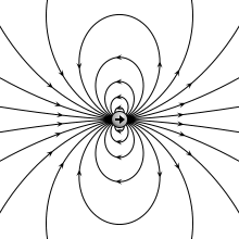
Рассчитанные электростатические поля четырёх различных типов электрических диполей.
1. Поле идеального точечного диполя. Конфигурация поля в большом масштабе инвариантна и приблизительно соответствует полю любой конфигурации зарядов с ненулевым дипольным моментом на большом расстоянии.
2. Дискретный диполь двух противоположно заряженных точечных зарядов разнесенных на конечное расстояние, — физический диполь.
3. Тонкий круглый диск с равномерной электрической поляризацией вдоль оси симметрии.
4. Плоский конденсатор с одинаково заряженными круглыми обкладками.
Несмотря на различие этих конфигураций, вблизи которых поля существенно различаются, все эти поля сходятся к одному и тому же дипольному полю на больших расстояниях, где они приблизительно одинаковы, при этом любая система зарядов может моделировать идеальный электрический диполь.

Простейшая система зарядов, имеющая определённый (не зависящий от выбора начала координат) ненулевой дипольный момент — диполь (две точечные частицы с одинаковыми по величине разноимёнными зарядами). Электрический дипольный момент такой системы по модулю равен произведению величины положительного заряда на расстояние между зарядами и направлен от отрицательного заряда к положительному, или:

{displaystyle mathbf {p} =qmathbf {l} ,}

где

— величина положительного заряда,

— вектор с началом в отрицательном заряде.

Для системы из частиц электрический дипольный момент равен:

${displaystyle mathbf {p} =sum _{i=1}^{N}q_{i}mathbf {r} _{i},}$

где $q_{i}$

— заряд частицы с номером

${mathbf r}_{i}$

— её радиус-вектор,

или, если суммировать отдельно по положительным и отрицательным зарядам:

${displaystyle mathbf {p} =sum _{i=1}^{N^{+}}q_{i}^{+}mathbf {r} _{i}-sum _{i=1}^{N^{-}}left|q_{i}^{-}right|r_{i}=Q^{+}mathbf {R} ^{+}-|Q^{-}|mathbf {R} ^{-},}$

где ${displaystyle N^{pm }}$

— число положительно/отрицательно заряженных частиц,

${displaystyle N=N^{+}~+N^{-},}$

${displaystyle q_{i}^{pm }}$

— их заряды,

${displaystyle Q^{+},~mathbf {R} ^{+},~Q^{-},~mathbf {R} ^{-}}$

— суммарные заряды положительной и отрицательной подсистем и радиус-векторы их «центров тяжести»^{[прим 2]}.

Электрический дипольный момент нейтральной системы зарядов не зависит от выбора начала координат, а определяется относительным расположением (и величинами) зарядов в системе.

Из определения видно, что дипольный момент аддитивен (дипольный момент наложения нескольких систем зарядов равен просто векторной сумме их дипольных моментов), а в случае нейтральных систем это свойство приобретает ещё более удобную форму в силу изложенного в абзаце выше.

Подробности определения и формальные свойства

Дипольный момент ненейтральной системы зарядов, вычисленный по приведенному выше определению, может выбором начала координат быть сделан равным любому наперед заданному числу (например, нулю). Однако и в этом случае, если мы хотим избежать такого произвола, при желании может быть использована какая-нибудь процедура внесения однозначности (которая будет тоже представлять собой предмет произвольного условного соглашения, но всё же будет формально фиксирована).

Но и при произвольном выборе начала координат (ограничивающемся тем условием, чтобы начало координат находилось внутри данной системы зарядов или, по крайней мере, близко от неё, и уж во всяком случае не попадая в ту область, в которой мы вычисляем дипольную поправку к полю единственного точечного заряда или дипольный член мультипольного разложения) все вычисления (дипольной поправки к потенциалу или напряженности поля, создаваемого системой, действующий на неё со стороны внешнего поля вращающий момент или дипольная поправка к потенциальной энергии системы во внешнем поле) проходят успешно.

Пример:

Интересной иллюстрацией мог бы быть следующий пример:

Рассмотрим систему, состоящую из единственного точечного заряда q, однако начало координат выберем не совпадающим с его положением, хотя и очень близко от него (т.е. много ближе, чем расстояние, для которого мы хотим вычислить потенциал, создаваемый этой нашей простой системой). Таким образом, радиус вектор нашего точечного заряда будет ${displaystyle {vec {r}}_{q};r_{q}<<r,}$ где r – модуль радиус-вектора точки наблюдения. Тогда формально нулевым приближением будет кулоновский потенциал ${displaystyle phi _{0}=q/r}$ ; однако это приближение содержит маленькую ошибку за счет того, что на самом деле расстояние от заряда до точки наблюдения не равно r, а равно ${displaystyle |mathbf {r} -mathbf {r} _{q}|}$ . Именно эту ошибку в первом порядке (т.е. тоже приближенно, но с лучшей точностью) исправляет добавление потенциала диполя с дипольным моментом, равным ${displaystyle qmathbf {r} _{q}}$ .
Наглядно это выглядит так: мы накладываем на заряд q, находящийся в начале координат, диполь так, что его отрицательный заряд -q в точности попадает на q в начале координат и его “уничтожает”, а его положительный заряд (+q) – попадает в точку ${displaystyle mathbf {r} _{q}}$ , то есть именно туда, где заряд должен находиться на самом деле – т.е. заряд передвигается из условного начала координат в правильное положение (хотя и близкое к началу координат). Используя суперпозицию дипольной поправки с нулевым приближением $phi _{0}$ , мы получаем более точный ответ, т.е. дипольная поправка в нашем примере вызывает эффект, (приближенно) эквивалентный тому, чтобы сдвинуть заряд из условного начала координат в его правильное положение.

Электрический дипольный момент (если он ненулевой) определяет в главном приближении электрическое^{[прим 3]} поле диполя (или любой ограниченной системы с суммарным нулевым зарядом) на большом расстоянии от него, а также воздействие на диполь внешнего электрического поля.

Физический и вычислительный смысл дипольного момента состоит в том, что он дает поправки первого порядка (чаще всего — малые) в положение каждого заряда системы по отношению к началу координат (которое может быть условным, но приближенно характеризует положение системы в целом — система при этом подразумевается достаточно компактной). Эти поправки входят в него в виде векторной суммы, и везде, где при вычислениях такая конструкция встречается (а в силу принципа суперпозиции и свойства сложения линейных поправок — см.Полный дифференциал — такая ситуация встречается часто), там в формулах оказывается дипольный момент.

Дипольный момент для атома с квантовой точки зрения[править | править код]

Из квантовой теории известно, что если система была в состоянии , то вероятность найти её в состоянии через время после вынужденного излучательного перехода под действием внешнего поля $E_{0}$ частотой будет равна:

${displaystyle a_{l}(t)={cfrac {|d_{kl}|^{2}}{4pi ^{2}}};E_{0}^{2};t;{cfrac {sin ^{2}(pi (nu -nu _{0})t)}{pi (nu -nu _{0})t}}.}$

Если наблюдать за системой продолжительное время, то последняя дробь в формуле перестаёт зависеть от времени, и выражение приведётся к виду:

${displaystyle a_{l}(t)={cfrac {|d_{kl}|^{2}}{4pi ^{2}}};E_{0}^{2};t;delta (nu -nu _{0}),}$

где ${displaystyle delta (nu -nu _{0})}$

— дельта-функция Дирака.

В указанной формуле ${displaystyle d_{kl}}$ — это элементы матричного оператора дипольного момента hat{d} по времени перехода которые определяются как:

${displaystyle d_{kl}=e;int _{V}Psi _{k}^{*}(x,y,z)cdot xcdot Psi _{l}(x,y,z);dV,}$

где

— заряд электрона,

— волновая функция (чётная либо нечётная).

В частности, очевидно, что если то интеграл станет равным нулю.

Соответственно, сам матричный оператор дипольного момента представляет собой матрицу размера [количество энергетических уровней умноженное на количество энергетических уровней], в которой элементы, лежащие на главной диагонали, равны нулю, а не лежащие — в общем случае не равны.

Электрическое поле диполя[править | править код]

Для фиксированных угловых координат (то есть вдоль радиуса, идущем из центра электрического диполя в бесконечность) напряжённость статического^{[прим 4]} электрического поля диполя или в целом нейтральной системы зарядов, имеющей ненулевой дипольный момент^{[прим 5]}, на больших расстояниях асимптотически приближается к виду ${displaystyle r^{-3},}$ электрический потенциал приближается к Таким образом, статическое поле диполя убывает на больших расстояниях быстрее, чем поле одиночного заряда, но медленнее, чем поле любого более старшего мультиполя (квадруполя, октуполя и т. д.).

Напряжённость электрического поля и электрический потенциал неподвижного или медленно движущегося диполя (или в целом нейтральной системы зарядов, имеющей ненулевой дипольный момент) с электрическим дипольным моментом на больших расстояниях в главном приближении выражаются как:

в СГСЭ: ${displaystyle mathbf {E} ={frac {3mathbf {n} (mathbf {n} cdot mathbf {p} )-mathbf {p} }{r^{3}}},qquad varphi =-mathbf {p} cdot mathbf {nabla } {frac {1}{r}},}$

в СИ: ${displaystyle mathbf {E} ={frac {3mathbf {n} (mathbf {n} cdot mathbf {p} )-mathbf {p} }{4pi varepsilon _{0}r^{3}}},qquad varphi =-mathbf {p} cdot mathbf {nabla } {frac {1}{4pi varepsilon _{0}r}},}$

где ${displaystyle mathbf {n} ={frac {mathbf {r} }{r}}}$

— единичный вектор из центра диполя в направлении точки измерения, а точкой обозначено скалярное произведение.

В декартовых координатах, ось которых направлена вдоль вектора дипольного момента, а ось выбрана так, чтобы точка, в которой рассчитывается поле, лежала в плоскости компоненты этого поля записываются так:

${displaystyle E_{x}={frac {p}{r^{3}}}(3cos ^{2}theta -1),}$

${displaystyle E_{y}={frac {3p}{r^{3}}}cos theta sin theta ,}$

${displaystyle E_{z}=0,}$

где

— угол между направлением вектора дипольного момента и радиус-вектором в точку наблюдения.

Формулы приведены в системе СГС. В СИ аналогичные формулы отличаются только множителем ${displaystyle {frac {1}{4pi varepsilon _{0}}}.}$

Достаточно просты выражения (в том же приближении, тождественно совпадающие с формулами, приведенными выше) для продольной (вдоль радиус-вектора, проведенного от диполя в данную точку) и поперечной компонент напряженности электрического поля:

${displaystyle E_{||}={frac {2p}{r^{3}}}cos theta ,}$

${displaystyle E_{perp }={frac {p}{r^{3}}}sin theta .}$

Третья компонента напряженности электрического поля — ортогональная плоскости, в которой лежат вектор дипольного момента и радиус-вектор, — всегда равна нулю. Формулы также в СГС, в СИ, как и формулы выше, отличаются лишь множителем ${displaystyle {frac {1}{4pi varepsilon _{0}}}.}$

Вывод

Имеем:

${displaystyle E_{||}=(mathbf {E} cdot mathbf {n} )={frac {3(mathbf {n} cdot mathbf {p} )-(mathbf {n} cdot mathbf {p} )}{r^{3}}}={frac {2(mathbf {n} cdot mathbf {p} )}{r^{3}}}={frac {2pcos theta }{r^{3}}},}$

Теперь:

${displaystyle mathbf {E_{perp }} =mathbf {E} -mathbf {n} E_{||}}$

Простой также оказывается связь угла между вектором и радиус-вектором (или вектором ):

${displaystyle mathrm {tg} beta ={frac {1}{2}}mathrm {tg} theta .}$

Модуль вектора напряженности электрического поля (в СГС):

${displaystyle E={frac {p}{r^{3}}}{sqrt {3cos ^{2}theta +1}}.}$

Действие поля на диполь[править | править код]

${displaystyle Sigma _{i}{frac {partial {mathbf {E} }}{partial x_{i}}}p_{i}.}$

Об условиях корректности приближенных (в общем случае) формул данного параграфа — см. ниже.

Единицы измерения электрического дипольного момента[править | править код]

Системные единицы измерения электрического дипольного момента не имеют специального названия. В Международной системе единиц (СИ) это просто Кл·м.

Электрический дипольный момент молекул принято измерять в дебаях (сокращение — Д):

1 Д = 10⁻¹⁸ единиц СГСЭ момента электрического диполя,

1 Д = 3,33564·10⁻³⁰ Кл·м.

Поляризация[править | править код]

Дипольный момент единицы объёма (поляризованной) среды (диэлектрика) называется вектором электрической поляризованности или просто поляризованностью диэлектрика.

Дипольный момент элементарных частиц[править | править код]

Многие экспериментальные работы посвящены поиску электрического дипольного момента (ЭДМ) фундаментальных и составных элементарных частиц, а именно электронов и нейтронов. Поскольку ЭДМ нарушает как пространственную (Р), так и временну́ю (T) чётность, его значение даёт (при условии ненарушенной СРТ-симметрии) модельно-независимую меру нарушения CP-симметрии в природе. Таким образом, значения ЭДМ дают сильные ограничения на масштаб CP-нарушения, которое может возникать в расширениях Стандартной Модели физики элементарных частиц.

Действительно, многие теории, несовместимые с существующими экспериментальными пределами на ЭДМ частиц, уже были исключены. Стандартная Модель (точнее, её раздел — квантовая хромодинамика) сама по себе допускает гораздо большее значение ЭДМ нейтрона (около 10⁻⁸ Д), чем эти пределы, что привело к возникновению так называемой сильной CP-проблеме и вызвало поиски новых гипотетических частиц, таких как аксион.

Текущие эксперименты по поиску ЭДМ частиц достигает чувствительности в диапазоне, где могут проявляться эффекты суперсимметрии. Эти эксперименты дополняют поиск эффектов суперсимметрии на LHC.

В 2018 г. установлено, что ЭДМ электрона не превышает ${displaystyle 1{,}1cdot 10^{-29}}$
e·см, e — элементарный заряд^[1].

Дипольное приближение[править | править код]

Дипольный член (определяемый дипольным моментом системы или распределения зарядов) является лишь одним из членов бесконечного ряда, называемого мультипольным разложением, дающего при полном суммировании точное значение потенциала или напряженности поля в точках, находящихся на конечном расстоянии от системы зарядов-источников. В этом смысле дипольный член выступает как равноправный с остальными, в том числе и высшими, членами мультипольного разложения (хотя зачастую он и может давать больший вклад в сумму, чем высшие члены). Этот взгляд на дипольный момент и дипольный вклад в создаваемое системой зарядов электрическое поле обладает существенной теоретической ценностью, но в деталях довольно сложен и довольно далеко выходит за рамки необходимого для понимания существенных физического смысла свойств дипольного момента и большинства областей его использования.

Для прояснения физического смысла дипольного момента, так же как и для большинства его приложений, достаточно ограничиться гораздо более простым подходом — рассматривать дипольное приближение.

Широкое использование дипольного приближения основывается на той ситуации, что очень во многих, в том числе теоретически и практически важных случаях, можно не суммировать весь ряд мультипольного разложения, а ограничиться только низшими его членами — до дипольного включительно. Часто этот подход дает вполне удовлетворительную или даже очень маленькую погрешность.

Дипольное приближение для системы источников[править | править код]

В электростатике достаточное условие применимости дипольного приближения (в смысле задачи определения электрического потенциала или напряженности электрического поля, создаваемого системой зарядов, имеющей определённый суммарный заряд и определённый дипольный момент) описывается весьма просто: хорошим это приближение является для областей пространства, удаленных от системы-источника на расстояние много большее, чем характерный (а лучше — чем максимальный) размер самой этой системы. Таким образом, для условий дипольное приближение является хорошим.

Если суммарный заряд системы равен нулю, а её дипольный момент нулю не равен, дипольное приближение в своей области применимости является главным приближением, то есть в его области применимости оно описывает основной вклад в электрическое поле. Остальные же вклады при пренебрежимо малы (если только дипольный момент не оказывается аномально малым, когда квадрупольный, октупольный или высшие мультипольные вклады на каких-то конечных расстояниях могут быть больше или сравнимы с дипольным; это однако достаточно специальный случай).

Если суммарный заряд не равен нулю, главным становится
монопольное приближение (нулевое приближение, закон Кулона в чистом виде), а дипольное приближение, являясь следующим, первым, приближением, может играть роль малой поправки к нему. Впрочем, в такой ситуации эта поправка будет очень мала в сравнении с нулевым приближением, если только мы находимся в области пространства, где вообще говоря само дипольное приближение является хорошим. Это несколько снижает его ценность в данном случае (за исключением, правда, ситуаций, описанных чуть ниже), поэтому главной областью применения дипольного приближения приходится признать случай нейтральных в целом систем зарядов.

Существуют ситуации, когда дипольное приближение является хорошим (иногда очень хорошим и в каких-то случаях даже может давать практически точное решение) и при невыполнении условия Для этого нужно только чтобы высшие мультипольные моменты (начиная с квадрупольного) обращались в ноль или очень быстро стремились к нулю. Это довольно легко реализуется для некоторых распределенных систем^{[прим 6]}

В дипольном приближении, если суммарный заряд ноль, вся система зарядов, какой бы она ни была, если только её дипольный момент не ноль, эквивалентна маленькому диполю (в этом случае всегда подразумевается маленький диполь) — в том смысле, что она создает поле, приближенно совпадающее с полем маленького диполя. В этом смысле любую такую систему отождествляют с диполем и к ней могут применяться термины диполь, поле диполя и т. д. В статье выше, даже если это не оговорено явно, всегда можно вместо слова диполь слова «нейтральная в целом система, имеющая ненулевой дипольный момент» — но, конечно, вообще говоря только в случае, если подразумевается выполнение условий корректности дипольного приближения.

Дипольное приближение для действия внешнего поля на систему зарядов[править | править код]

Идеально дипольное приближение для формул механического момента, создаваемого внешним полем, действующим на диполь, и потенциальной энергии диполя во внешнем поле, работает в случае однородности внешнего поля. В этом случае эти две формулы выполняются точно для любой системы, имеющей определённый дипольный момент, независимо от размера (равенство нулю суммарного её заряда подразумевается).

Границу приемлемости дипольного приближения для этих формул определяет в целом такое условие: разность напряженности поля в разных точках системы должна быть по модулю много меньше самого значения напряженности поля. Качественно это означает, что для обеспечения корректности этих формул размеры системы должны быть тем меньше, чем более неоднородно действующее на неё поле.

Примечания[править | править код]

Комментарии

↑ То есть, самый старший после нулевого мультипольного момента, равного полному заряду системы.
↑ Под радиус векторами «центров тяжести» тут имеется в виду средневзвешенные значение радиус-вектора по каждой из подсистем, где каждому заряду приписывается формальный вес, равный абсолютной величине этого заряда.
↑ Для достаточно быстро колеблющегося электрического диполя его дипольный момент (с его зависимостью от времени) определяет также и магнитное поле. Неподвижный электрический диполь не создаёт магнитное поле (это приближенно верно и для медленно движущегося диполя).
↑ Здесь описывается поле неподвижного или (приближенно) медленно движущегося диполя.
↑ Поле такой системы на большом расстоянии приближенно равно полю одного диполя. В этом смысле такую систему можно (приближенно) заменить на диполь и рассматривать как идеальный диполь.
↑ . Одним из простых примеров такой системы является наложение двух одинаковых шаров, равномерно заряженных одинаковыми по абсолютной величине зарядами разного знака, причем расстояние между центрами шаров мало. Поле такой системы уже вблизи её поверхности очень хорошо совпадает с полем (маленького) диполя. Такое же поле дает похожая система, состоящая из сферы, поверхность которой заряжена с плотностью заряда, пропорциональной косинусу широты на сфере. Можно специально подобрать непрерывные распределения зарядов и в других телах или на поверхностях, дающие поле диполя. В некоторых случаях это происходит автоматически: например, точечный заряд (или маленький равномерно заряженный шар), расположенный вблизи большой металлической плоскости, создает на ней такой распределение поверхностного заряда, что вся система в целом создает поле диполя даже совсем вблизи плоскости (но не рядом с шаром и вдали от края плоскости, если она не бесконечная).

Источники

↑ ACME Collaboration Improved limit on the electric dipole moment of the electron // Nature, volume 562, pages 355—360, (2018)

Литература[править | править код]

Ландау Л. Д., Лифшиц Е. М. Теория поля. — Издание 7-е, исправленное. — М.: Наука, 1988. — 512 с. — («Теоретическая физика», том II). — ISBN 5-02-014420-7.
Минкин В. И., Осипов О. А., Жданов Ю. А., Дипольные моменты в органической химии. Л., 1968;
Осипов О. А., Минкин В. И., Гарновский А. Д., Справочник по дипольным моментам, 3 изд.. М., 1971;
Exner О., Dipole moments in organic chemistry, Stuttg., 1975.

Источник

3.1 Дипольный момент системы зарядов, поляризация диэлектриков

Рассмотрим систему произвольного числа зарядов, притом такую, что суммарный алгебраический заряд её равен нулю `sum_iq_i=0`. Пусть система состоит из `N` точечных зарядов произвольной величины `q_i(i=1,2,3,…N)` и пусть в некоторой системе координат каждый из зарядов характеризуется своим радиус-вектором `vecr_i`. По определению электрическим дипольным моментом системы называют вектор

`vecp=sum_iq_ivecr_i`. (3.1.1)

Электрические свойства диэлектриков обусловлены реакцией на внешнее поле не свободных электронов, как в металлах (в диэлектриках свободных электронов чрезвычайно мало), а так называемых связанных электронов – связанных с отдельными диполями молекул диэлектрика. Надо сразу сказать, что молекулы (атомы) разных веществ бывают двух сортов. Первые из них уже без всякого внешнего поля имеют дипольные моменты (например, молекулы воды); такие молекулы называют полярными, а вместе с ними и сами диэлектрики называют полярными. У другого сорта диэлектриков дипольный момент молекул в отсутствие внешнего поля равен нулю (например, в симметричных молекулах `”O”_2`, `”N”_2`, `”CO”_2`); такие молекулы называют неполярными; соответственно и диэлектрики, состоящие из таких молекул называют неполярными.

В отсутствие внешнего электрического поля даже вещества с полярными молекулами, как правило, никак себя электрически не проявляют. Это связано с тем, что диполи различных молекул в них направлены совершенно хаотически и, «действуя не согласованно», не создают никакого суммарного макроскопического электрического поля.

При помещении во внешнее электрическое поле (везде далее будем считать это поле однородным) вещества двух указанных сортов ведут себя в чём-то по-разному, но в чём-то и схоже. В полярных диэлектриках в расположении (ориентации) диполей появляется упорядоченность – диполи молекул стремятся выстроиться преимущественно по полю.

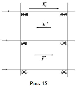
В неполярных диэлектриках электронные облака молекул деформируются так, что у них появляются индивидуальные дипольные моменты, которые также стремятся выстроиться преимущественно по полю – говорят, что происходит поляризация диэлектриков. В результате в обоих случаях на границах диэлектрика появляются, как и в металлах, избыточные поверхностные заряды той же полярности, что и в металлах. Наведённое ими электрическое поле `E^’` также направлено на встречу внешнему полю `E_0`, а суммарное поле `E=E_0-E^’` меньше внешнего (рис. 15). В проводниках в статических условиях это поле не просто меньше внешнего, но в точности равно нулю. В диэлектриках оно до нуля не ослабляется, оставаясь конечным и равным `E=E_0//epsilon`. Где `epsilon` – так называемая диэлектрическая проницаемость среды, показывающая во сколько раз диэлектрик ослабляет внешнее электрическое поле.

Простое ослабление внешнего поля в диэлектрике в `epsilon` раз относится лишь к простейшей геометрии опыта, когда внешнее электрическое поле перпендикулярно поверхности диэлектрика. Рассмотрение случаев, когда поле направлено под другими углами к поверхности, выходит за рамки настоящего Задания.

Какие порядки величин `epsilon` встречаются? Для воздуха (и вообще, для газов, т. е. довольно разреженных систем с неполярными молекулами) эта величина лишь ненамного превосходит единицу: `epsilon~~1,00058`. А вот для воды эта величина значительно больше: `epsilon~~81`. Последнее связано с тем, что, во-первых, молекулы воды `”H”_2″O”` суть полярные молекулы (электроны в них смещены от атомов водорода к атому кислороду), а во-вторых, концентрация молекул в воде значительно больше, чем в воздухе.

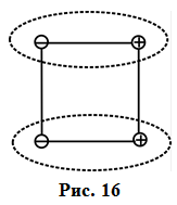
Заряды `+q,+q,-q` и `-q` расположены последовательно в вершинах квадрата, если обходить его по часовой стрелке. Сторона квадрата равна `l`. Определить дипольный момент системы.

Рассмотрим две пары разноимённо заряженных зарядов (рис. 16). В каждой паре дипольный момент будет равен по модулю величине `ql`, и для разных пар дипольные моменты направлены в одну и ту же сторону, поэтому их сумма равна `2ql`.

Металлический шар радиусом `R` с зарядом `Q` находится в среде с диэлектрической проницаемостью `epsilon`. Определить суммарный заряд `Q^’` связанных зарядов на поверхности шара.

Ослабление в `epsilon` раз поля шара с зарядом `Q` обусловлено тем, что не его поверхности появляется заряд `Q^’`: `1/(epsilon) Q/(4pi epsilon_0r^2)=(Q+Q^’)/(4pi epsilon_0r^2)`, откуда `Q^’=-(epsilon-1)/(epsilon)Q`.

Источник

Теоретическая часть.

§1. Электрический диполь. Электрический дипольный момент.

Электрическим
диполем
называется система двух отличающихся
только знаком точечных зарядов +q
и -q
, расстояние

между которыми мало по сравнению с
расстоянием до тех точек, в которых
рассматривается поле системы. Прямая,
проходящая через оба заряда, называется
осью
диполя.
Плечом
диполя называется вектор
,
направленный по оси диполя от отрицательного
заряда к положительному и по модулю
равный расстоянию между ними.

рис.
1

Произведение
положительного заряда диполя на плечо
называется электрическим
моментом диполя
(дипольным электрическим моментом):

.
(1.1)

Напряженность
поля диполя:

где
p – электрический момент диполя; r –
модуль радиус-вектора, проведенного от
центра диполя к точке, напряженность в
которой нас интересует; α – угол между
радиус-вектором
и
плечом диполя
.

рис.
2

Напряженности
на оси диполя (α= 0) и в точке, лежащей на
перпендикуляре к плечу диполя,
восстановленному из его середины (α =
), соответственно равны:

Потенциал
поля в точке можно вычислить по формуле:

§2. Диполь в однородном и неоднородном электрическом поле. Момент сил, действующий на диполь в электрическом поле.

Однородное
внешнее поле:

Поместим
диполь во внешнее однородное поле.
Полная сила, действующая на диполь,
очевидно, равна нулю, из-за того, что
силы, действующие на каждый из зарядов,
различны по знаку, но одинаковы по
модулю:

Поэтому
диполь в однородном поле не смещается.
Однако на диполь

действует
пара сил на расстоянии (плечо пары сил)

, где угол 𝜃
–

угол
между направлением вектора напряженности
поля и дипольным

моментом.
Откуда:

Следовательно,
момент силы, стремящийся повернуть
дипольный момент вдоль направления
поля, отличен от нуля:

(2.3)

Наиболее
устойчивое положение диполя возникает
тогда, когда вектор дипольного момента
направлен вдоль вектора напряженности
электрического поля. В противном случае
(вектор

противоположно направлен вектору
напряженности), положение равновесия
неустойчиво.

Следовательно,
в однородном внешнем электрическом
поле диполь поворачивается и располагается
так, чтобы его дипольный момент был
ориентирован по полю.

В
неоднородном поле кроме механического
момента на точечный диполь действует
сила F,
которая выталкивает (или втягивает)
диполь из поля. В случае поля обладающего,
симметрией относительно оси ОХ, сила
выражается соотношением:

§3. Полярные и неполярные диэлектрики.

Диэлектриками
(или изоляторами) называются вещества,
не способные проводить электрический
ток.

Молекулы
диэлектрика представляют собой
электрические диполи. В отсутствии
внешнего электрического поля вследствие
хаотического теплового движения
суммарное поле всех молекул–диполей
равно нулю.

У
диэлектриков заряды, входящие в состав
молекулы, прочно связаны друг с другом
и могут быть разъединены только при
воздействии на них очень сильного поля.
Поэтому заряды, входящие в состав молекул
диэлектрика, называются связанными.
Под действием внешнего поля связанные
заряды разных знаков лишь немного
смещаются в противоположные стороны;
покинуть пределы молекул, в состав
которой они входят, связанные заряды
не могут.

Внутри
или на поверхности диэлектрика могут
находиться заряды, который не входят в
состав его молекул. Такие заряды, а также
заряды, расположенные за пределами
диэлектрика, называются сторонними.

По
механизмам поляризации молекул различают
полярные и неполярные диэлектрики.

Неполярные
диэлектрики (нейтральные) – состоят из
неполярных молекул, у которых центры
тяжести положительного и отрицательного
зарядов совпадают. Следовательно,
неполярные молекулы не обладают
электрическим моментом и их электрический
момент равен нулю. Примером
практически неполярных диэлектриков,
применяемых в качестве электроизоляционных,
являются углеводородные материалы,
нефтяные электроизоляционные масла,
полиэтилен, полистирол и др.

Полярные
диэлектрики (дипольные) – состоят из
полярных молекул, обладающих электрическим
моментом. В таких молекулах из-за их
асимметричного строения центры масс
положительных и отрицательных зарядов
не совпадают. К
полярным диэлектрикам относятся
фенолоформальдегидные и эпоксидные
смолы, кремнийорганические соединения,
хлорированные углеводороды и др.

Соседние файлы в предмете [НЕСОРТИРОВАННОЕ]

Источник

The electric field due to a point dipole (upper left), a physical dipole of electric charges (upper right), a thin polarized sheet (lower left) or a plate capacitor (lower right). All generate the same field profile when the arrangement is infinitesimally small.

The electric dipole moment is a measure of the separation of positive and negative electrical charges within a system, that is, a measure of the system’s overall polarity. The SI unit for electric dipole moment is the coulomb-meter (C⋅m). The debye (D) is another unit of measurement used in atomic physics and chemistry.

Theoretically, an electric dipole is defined by the first-order term of the multipole expansion; it consists of two equal and opposite charges that are infinitesimally close together, although real dipoles have separated charge.^{[notes 1]}

Elementary definition[edit]

Quantities defining the electric dipole moment of two point charges.

Animation showing the electric field of an electric dipole. The dipole consists of two point electric charges of opposite polarity located close together. A transformation from a point-shaped dipole to a finite-size electric dipole is shown.

A molecule of water is polar because of the unequal sharing of its electrons in a “bent” structure. A separation of charge is present with negative charge in the middle (red shade), and positive charge at the ends (blue shade).

Often in physics the dimensions of a massive object can be ignored and can be treated as a pointlike object, i.e. a point particle. Point particles with electric charge are referred to as point charges. Two point charges, one with charge +q and the other one with charge −q separated by a distance d, constitute an electric dipole (a simple case of an electric multipole). For this case, the electric dipole moment has a magnitude

and is directed from the negative charge to the positive one. Some authors may split d in half and use s = d/2 since this quantity is the distance between either charge and the center of the dipole, leading to a factor of two in the definition.

A stronger mathematical definition is to use vector algebra, since a quantity with magnitude and direction, like the dipole moment of two point charges, can be expressed in vector form

where d is the displacement vector pointing from the negative charge to the positive charge. The electric dipole moment vector p also points from the negative charge to the positive charge. With this definition the dipole direction tends to align itself with an external electric field (and note that the electric flux lines produced by the charges of the dipole itself, which point from positive charge to negative charge then tend to oppose the flux lines of the external field). Note that this sign convention is used in physics, while the opposite sign convention for the dipole, from the positive charge to the negative charge, is used in chemistry.^[1]

An idealization of this two-charge system is the electrical point dipole consisting of two (infinite) charges only infinitesimally separated, but with a finite p. This quantity is used in the definition of polarization density.

Energy and torque[edit]

Electric dipole p and its torque τ in a uniform E field.

An object with an electric dipole moment p is subject to a torque τ when placed in an external electric field E. The torque tends to align the dipole with the field. A dipole aligned parallel to an electric field has lower potential energy than a dipole making some angle with it. For a spatially uniform electric field across the small region occupied by the dipole, the energy U and the torque are given by^[2]

The scalar dot “⋅” product and the negative sign shows the potential energy minimises when the dipole is parallel with field and is maximum when antiparallel while zero when perpendicular. The symbol “×” refers to the vector cross product. The E-field vector and the dipole vector define a plane, and the torque is directed normal to that plane with the direction given by the right-hand rule. Note that a dipole in such a uniform field may twist and oscillate but receives no overall net force with no linear acceleration of the dipole. The dipole twists to align with the external field.

However in a non-uniform electric field a dipole may indeed receive a net force since the force on one end of the dipole no longer balances that on the other end. It can be shown that this net force is generally parallel to the dipole moment.

Expression (general case)[edit]

More generally, for a continuous distribution of charge confined to a volume V, the corresponding expression for the dipole moment is:

${displaystyle mathbf {p} (mathbf {r} )=int _{V}rho (mathbf {r} ')left(mathbf {r} '-mathbf {r} right)d^{3}mathbf {r} ',}$

where r locates the point of observation and d³r′ denotes an elementary volume in V. For an array of point charges, the charge density becomes a sum of Dirac delta functions:

${displaystyle rho (mathbf {r} )=sum _{i=1}^{N},q_{i},delta left(mathbf {r} -mathbf {r} _{i}right),}$

where each r_i is a vector from some reference point to the charge q_i. Substitution into the above integration formula provides:

${displaystyle mathbf {p} (mathbf {r} )=sum _{i=1}^{N},q_{i}int _{V}delta left(mathbf {r} _{0}-mathbf {r} _{i}right),left(mathbf {r} _{0}-mathbf {r} right),d^{3}mathbf {r} _{0}=sum _{i=1}^{N},q_{i}left(mathbf {r} _{i}-mathbf {r} right).}$

This expression is equivalent to the previous expression in the case of charge neutrality and N = 2. For two opposite charges, denoting the location of the positive charge of the pair as r₊ and the location of the negative charge as r₋:

${displaystyle mathbf {p} (mathbf {r} )=q_{1}(mathbf {r} _{1}-mathbf {r} )+q_{2}(mathbf {r} _{2}-mathbf {r} )=q(mathbf {r} _{+}-mathbf {r} )-q(mathbf {r} _{-}-mathbf {r} )=q(mathbf {r} _{+}-mathbf {r} _{-})=qmathbf {d} ,}$

showing that the dipole moment vector is directed from the negative charge to the positive charge because the position vector of a point is directed outward from the origin to that point.

The dipole moment is particularly useful in the context of an overall neutral system of charges, for example a pair of opposite charges, or a neutral conductor in a uniform electric field.
For such a system of charges, visualized as an array of paired opposite charges, the relation for electric dipole moment is:

${displaystyle {begin{aligned}mathbf {p} (mathbf {r} )&=sum _{i=1}^{N},int _{V}q_{i}left[delta left(mathbf {r} _{0}-left(mathbf {r} _{i}+mathbf {d} _{i}right)right)-delta left(mathbf {r} _{0}-mathbf {r} _{i}right)right],left(mathbf {r} _{0}-mathbf {r} right) d^{3}mathbf {r} _{0}\&=sum _{i=1}^{N},q_{i},left[mathbf {r} _{i}+mathbf {d} _{i}-mathbf {r} -left(mathbf {r} _{i}-mathbf {r} right)right]\&=sum _{i=1}^{N}q_{i}mathbf {d} _{i}=sum _{i=1}^{N}mathbf {p} _{i},,end{aligned}}}$

where r is the point of observation, and d_i = r‘_i − r_i, r_i being the position of the negative charge in the dipole i, and r‘_i the position of the positive charge.
This is the vector sum of the individual dipole moments of the neutral charge pairs. (Because of overall charge neutrality, the dipole moment is independent of the observer’s position r.) Thus, the value of p is independent of the choice of reference point, provided the overall charge of the system is zero.

When discussing the dipole moment of a non-neutral system, such as the dipole moment of the proton, a dependence on the choice of reference point arises. In such cases it is conventional to choose the reference point to be the center of mass of the system, not some arbitrary origin.^[3] This choice is not only a matter of convention: the notion of dipole moment is essentially derived from the mechanical notion of torque, and as in mechanics, it is computationally and theoretically useful to choose the center of mass as the observation point. For a charged molecule the center of charge should be the reference point instead of the center of mass. For neutral systems the reference point is not important, and the dipole moment is an intrinsic property of the system.

Potential and field of an electric dipole[edit]

Potential map of a physical electric dipole. Negative potentials are in blue; positive potentials, in red.

An ideal dipole consists of two opposite charges with infinitesimal separation. We compute the potential and field of such an ideal dipole starting with two opposite charges at separation d > 0, and taking the limit as d → 0.

Two closely spaced opposite charges ±q have a potential of the form:

${displaystyle phi (mathbf {r} ) = {frac {1}{4pi varepsilon _{0}}}left({frac {q}{left|mathbf {r} -mathbf {r} _{+}right|}}-{frac {q}{left|mathbf {r} -mathbf {r} _{-}right|}}right),}$

corresponding to the charge density

${displaystyle rho (mathbf {r} ) = -varepsilon _{0}nabla ^{2}phi = qdelta left(mathbf {r} -mathbf {r} _{+}right)-qdelta left(mathbf {r} -mathbf {r} _{-}right)}$

by Coulomb’s law,
where the charge separation is:

${displaystyle mathbf {d} =mathbf {r} _{+}-mathbf {r} _{-},,quad d=|mathbf {d} |,.}$

Let R denote the position vector relative to the midpoint ${displaystyle {frac {mathbf {r} _{+}+mathbf {r} _{-}}{2}}}$ , and the corresponding unit vector:

${displaystyle mathbf {R} =mathbf {r} -{frac {mathbf {r} _{+}+mathbf {r} _{-}}{2}},quad {hat {mathbf {R} }}={frac {mathbf {R} }{R}},,}$

Taylor expansion in ${displaystyle {tfrac {d}{R}}}$ (see multipole expansion and quadrupole) expresses this potential as a series.^[4]^[5]

${displaystyle phi (mathbf {R} ) = {frac {1}{4pi varepsilon _{0}}}{frac {qmathbf {d} cdot {hat {mathbf {R} }}}{R^{2}}}+{mathcal {O}}left({frac {d^{3}}{R^{3}}}right) approx {frac {1}{4pi varepsilon _{0}}}{frac {mathbf {p} cdot {hat {mathbf {R} }}}{R^{2}}},,}$

where higher order terms in the series are vanishing at large distances, R, compared to d.^{[notes 2]} Here, the electric dipole moment p is, as above:

The result for the dipole potential also can be expressed as:^[7]

${displaystyle phi (mathbf {R} )approx -mathbf {p} cdot mathbf {nabla } {frac {1}{4pi varepsilon _{0}R}},,}$

which relates the dipole potential to that of a point charge. A key point is that the potential of the dipole falls off faster with distance R than that of the point charge.

The electric field of the dipole is the negative gradient of the potential, leading to:^[7]

${displaystyle mathbf {E} left(mathbf {R} right)={frac {3left(mathbf {p} cdot {hat {mathbf {R} }}right){hat {mathbf {R} }}-mathbf {p} }{4pi varepsilon _{0}R^{3}}},.}$

Thus, although two closely spaced opposite charges are not quite an ideal electric dipole (because their potential at short distances is not that of a dipole), at distances much larger than their separation, their dipole moment p appears directly in their potential and field.

As the two charges are brought closer together (d is made smaller), the dipole term in the multipole expansion based on the ratio d/R becomes the only significant term at ever closer distances R, and in the limit of infinitesimal separation the dipole term in this expansion is all that matters. As d is made infinitesimal, however, the dipole charge must be made to increase to hold p constant. This limiting process results in a “point dipole”.

Dipole moment density and polarization density[edit]

The dipole moment of an array of charges,

${displaystyle mathbf {p} =sum _{i=1}^{N}q_{i}mathbf {d_{i}} ,,}$

determines the degree of polarity of the array, but for a neutral array it is simply a vector property of the array with no information about the array’s absolute location. The dipole moment density of the array p(r) contains both the location of the array and its dipole moment. When it comes time to calculate the electric field in some region containing the array, Maxwell’s equations are solved, and the information about the charge array is contained in the polarization density P(r) of Maxwell’s equations. Depending upon how fine-grained an assessment of the electric field is required, more or less information about the charge array will have to be expressed by P(r). As explained below, sometimes it is sufficiently accurate to take P(r) = p(r). Sometimes a more detailed description is needed (for example, supplementing the dipole moment density with an additional quadrupole density) and sometimes even more elaborate versions of P(r) are necessary.

It now is explored just in what way the polarization density P(r) that enters Maxwell’s equations is related to the dipole moment p of an overall neutral array of charges, and also to the dipole moment density p(r) (which describes not only the dipole moment, but also the array location). Only static situations are considered in what follows, so P(r) has no time dependence, and there is no displacement current. First is some discussion of the polarization density P(r). That discussion is followed with several particular examples.

A formulation of Maxwell’s equations based upon division of charges and currents into “free” and “bound” charges and currents leads to introduction of the D– and P-fields:

${displaystyle mathbf {D} =varepsilon _{0}mathbf {E} +mathbf {P} ,,}$

where P is called the polarization density. In this formulation, the divergence of this equation yields:

${displaystyle nabla cdot mathbf {D} =rho _{f}=varepsilon _{0}nabla cdot mathbf {E} +nabla cdot mathbf {P} ,,}$

and as the divergence term in E is the total charge, and ρ_f is “free charge”, we are left with the relation:

${displaystyle nabla cdot mathbf {P} =-rho _{b},,}$

with ρ_b as the bound charge, by which is meant the difference between the total and the free charge densities.

As an aside, in the absence of magnetic effects, Maxwell’s equations specify that

which implies

Applying Helmholtz decomposition:^[8]

for some scalar potential φ, and:

${displaystyle nabla cdot (mathbf {D} -mathbf {P} )=varepsilon _{0}nabla cdot mathbf {E} =rho _{f}+rho _{b}=-nabla ^{2}varphi ,.}$

Suppose the charges are divided into free and bound, and the potential is divided into

${displaystyle varphi =varphi _{f}+varphi _{b},.}$

Satisfaction of the boundary conditions upon φ may be divided arbitrarily between φ_f and φ_b because only the sum φ must satisfy these conditions. It follows that P is simply proportional to the electric field due to the charges selected as bound, with boundary conditions that prove convenient.^{[notes 3]}^{[notes 4]} In particular, when no free charge is present, one possible choice is P = ε₀ E.

Next is discussed how several different dipole moment descriptions of a medium relate to the polarization entering Maxwell’s equations.

Medium with charge and dipole densities[edit]

As described next, a model for polarization moment density p(r) results in a polarization

restricted to the same model. For a smoothly varying dipole moment distribution p(r), the corresponding bound charge density is simply

${displaystyle nabla cdot mathbf {p} (mathbf {r} )=-rho _{b},}$

as we will establish shortly via integration by parts. However, if p(r) exhibits an abrupt step in dipole moment at a boundary between two regions, ∇·p(r) results in a surface charge component of bound charge. This surface charge can be treated through a surface integral, or by using discontinuity conditions at the boundary, as illustrated in the various examples below.

As a first example relating dipole moment to polarization, consider a medium made up of a continuous charge density ρ(r) and a continuous dipole moment distribution p(r).^{[notes 5]} The potential at a position r is:^[10]^[11]

${displaystyle phi (mathbf {r} )={frac {1}{4pi varepsilon _{0}}}int {frac {rho left(mathbf {r} _{0}right)}{left|mathbf {r} -mathbf {r} _{0}right|}}d^{3}mathbf {r} _{0} +{frac {1}{4pi varepsilon _{0}}}int {frac {mathbf {p} left(mathbf {r} _{0}right)cdot left(mathbf {r} -mathbf {r} _{0}right)}{|mathbf {r} -mathbf {r} _{0}|^{3}}}d^{3}mathbf {r} _{0},}$

where ρ(r) is the unpaired charge density, and p(r) is the dipole moment density.^{[notes 6]} Using an identity:

${displaystyle nabla _{mathbf {r} _{0}}{frac {1}{left|mathbf {r} -mathbf {r} _{0}right|}}={frac {mathbf {r} -mathbf {r} _{0}}{left|mathbf {r} -mathbf {r} _{0}right|^{3}}}}$

the polarization integral can be transformed:

${displaystyle {begin{aligned}{frac {1}{4pi varepsilon _{0}}}int {frac {mathbf {p} left(mathbf {r} _{0}right)cdot (mathbf {r} -mathbf {r} _{0})}{left|mathbf {r} -mathbf {r} _{0}right|^{3}}}d^{3}mathbf {r} _{0}={}&{frac {1}{4pi varepsilon _{0}}}int mathbf {p} left(mathbf {r} _{0}right)cdot nabla _{mathbf {r} _{0}}{frac {1}{left|mathbf {r} -mathbf {r} _{0}right|}}d^{3}mathbf {r} _{0},\={}&{frac {1}{4pi varepsilon _{0}}}int nabla _{mathbf {r} _{0}}cdot left(mathbf {p} left(mathbf {r} _{0}right){frac {1}{left|mathbf {r} -mathbf {r} _{0}right|}}right)d^{3}mathbf {r} _{0}-{frac {1}{4pi varepsilon _{0}}}int {frac {nabla _{mathbf {r} _{0}}cdot mathbf {p} left(mathbf {r} _{0}right)}{left|mathbf {r} -mathbf {r} _{0}right|}}d^{3}mathbf {r} _{0},end{aligned}}}$

where the vector identity

was used in the last steps. The first term can be transformed to an integral over the surface bounding the volume of integration, and contributes a surface charge density, discussed later. Putting this result back into the potential, and ignoring the surface charge for now:

${displaystyle phi (mathbf {r} )={frac {1}{4pi varepsilon _{0}}}int {frac {rho left(mathbf {r} _{0}right)-nabla _{mathbf {r} _{0}}cdot mathbf {p} left(mathbf {r} _{0}right)}{left|mathbf {r} -mathbf {r} _{0}right|}}d^{3}mathbf {r} _{0},,}$

where the volume integration extends only up to the bounding surface, and does not include this surface.

The potential is determined by the total charge, which the above shows consists of:

${displaystyle rho _{text{total}}left(mathbf {r} _{0}right)=rho left(mathbf {r} _{0}right)-nabla _{mathbf {r} _{0}}cdot mathbf {p} left(mathbf {r} _{0}right),,}$

showing that:

${displaystyle -nabla _{mathbf {r} _{0}}cdot mathbf {p} left(mathbf {r} _{0}right)=rho _{b},.}$

In short, the dipole moment density p(r) plays the role of the polarization density P for this medium. Notice, p(r) has a non-zero divergence equal to the bound charge density (as modeled in this approximation).

It may be noted that this approach can be extended to include all the multipoles: dipole, quadrupole, etc.^[12]^[13] Using the relation:

${displaystyle nabla cdot mathbf {D} =rho _{f},,}$

the polarization density is found to be:

${displaystyle mathbf {P} (mathbf {r} )=mathbf {p} _{text{dip}}-nabla cdot mathbf {p} _{text{quad}}+cdots ,,}$

where the added terms are meant to indicate contributions from higher multipoles. Evidently, inclusion of higher multipoles signifies that the polarization density P no longer is determined by a dipole moment density p alone. For example, in considering scattering from a charge array, different multipoles scatter an electromagnetic wave differently and independently, requiring a representation of the charges that goes beyond the dipole approximation.^[14]^[15]

Surface charge[edit]

A uniform array of identical dipoles is equivalent to a surface charge.

Above, discussion was deferred for the first term in the expression for the potential due to the dipoles. Integrating the divergence results in a surface charge. The figure at the right provides an intuitive idea of why a surface charge arises. The figure shows a uniform array of identical dipoles between two surfaces. Internally, the heads and tails of dipoles are adjacent and cancel. At the bounding surfaces, however, no cancellation occurs. Instead, on one surface the dipole heads create a positive surface charge, while at the opposite surface the dipole tails create a negative surface charge. These two opposite surface charges create a net electric field in a direction opposite to the direction of the dipoles.

This idea is given mathematical form using the potential expression above. Ignoring the free charge, the potential is:

${displaystyle phi left(mathbf {r} right)={frac {1}{4pi varepsilon _{0}}}int nabla _{mathbf {r} _{0}}cdot left(mathbf {p} left(mathbf {r} _{0}right){frac {1}{left|mathbf {r} -mathbf {r} _{0}right|}}right)d^{3}mathbf {r} _{0}-{frac {1}{4pi varepsilon _{0}}}int {frac {nabla _{mathbf {r} _{0}}cdot mathbf {p} left(mathbf {r} _{0}right)}{left|mathbf {r} -mathbf {r} _{0}right|}}d^{3}mathbf {r} _{0},.}$

Using the divergence theorem, the divergence term transforms into the surface integral:

${displaystyle {frac {1}{4pi varepsilon _{0}}}int nabla _{mathbf {r} _{0}}cdot left(mathbf {p} left(mathbf {r} _{0}right){frac {1}{left|mathbf {r} -mathbf {r} _{0}right|}}right)d^{3}mathbf {r} _{0}={frac {1}{4pi varepsilon _{0}}}int {frac {mathbf {p} left(mathbf {r} _{0}right)cdot dmathbf {A} _{0}}{left|mathbf {r} -mathbf {r} _{0}right|}},,}$

with dA₀ an element of surface area of the volume. In the event that p(r) is a constant, only the surface term survives:

${displaystyle phi (mathbf {r} )={frac {1}{4pi varepsilon _{0}}}int {frac {1}{left|mathbf {r} -mathbf {r} _{0}right|}} mathbf {p} cdot dmathbf {A} _{0},,}$

with dA₀ an elementary area of the surface bounding the charges. In words, the potential due to a constant p inside the surface is equivalent to that of a surface charge

which is positive for surface elements with a component in the direction of p and negative for surface elements pointed oppositely. (Usually the direction of a surface element is taken to be that of the outward normal to the surface at the location of the element.)

If the bounding surface is a sphere, and the point of observation is at the center of this sphere, the integration over the surface of the sphere is zero: the positive and negative surface charge contributions to the potential cancel. If the point of observation is off-center, however, a net potential can result (depending upon the situation) because the positive and negative charges are at different distances from the point of observation.^{[notes 7]} The field due to the surface charge is:

${displaystyle mathbf {E} left(mathbf {r} right)=-{frac {1}{4pi varepsilon _{0}}}nabla _{mathbf {r} }int {frac {1}{left|mathbf {r} -mathbf {r} _{0}right|}} mathbf {p} cdot dmathbf {A} _{0},,}$

which, at the center of a spherical bounding surface is not zero (the fields of negative and positive charges on opposite sides of the center add because both fields point the same way) but is instead:^[17]

${displaystyle mathbf {E} =-{frac {mathbf {p} }{3varepsilon _{0}}},.}$

If we suppose the polarization of the dipoles was induced by an external field, the polarization field opposes the applied field and sometimes is called a depolarization field.^[18]^[19] In the case when the polarization is outside a spherical cavity, the field in the cavity due to the surrounding dipoles is in the same direction as the polarization.^{[notes 8]}

In particular, if the electric susceptibility is introduced through the approximation:

${displaystyle mathbf {p} (mathbf {r} )=varepsilon _{0}chi (mathbf {r} )mathbf {E} (mathbf {r} ),,}$

where E, in this case and in the following, represent the external field which induces the polarization.

Then:

${displaystyle nabla cdot mathbf {p} (mathbf {r} )=nabla cdot left(chi (mathbf {r} )varepsilon _{0}mathbf {E} (mathbf {r} )right)=-rho _{b},.}$

Whenever χ(r) is used to model a step discontinuity at the boundary between two regions, the step produces a surface charge layer. For example, integrating along a normal to the bounding surface from a point just interior to one surface to another point just exterior:

${displaystyle varepsilon _{0}{hat {mathbf {n} }}cdot left[chi left(mathbf {r} _{+}right)mathbf {E} left(mathbf {r} _{+}right)-chi left(mathbf {r} _{-}right)mathbf {E} left(mathbf {r} _{-}right)right]={frac {1}{A_{n}}}int dOmega _{n} rho _{b}=0,,}$

where A_n, Ω_n indicate the area and volume of an elementary region straddling the boundary between the regions, and a unit normal to the surface. The right side vanishes as the volume shrinks, inasmuch as ρ_b is finite, indicating a discontinuity in E, and therefore a surface charge. That is, where the modeled medium includes a step in permittivity, the polarization density corresponding to the dipole moment density

necessarily includes the contribution of a surface charge.^[21]^[22]^[23]

A physically more realistic modeling of p(r) would have the dipole moment density drop off rapidly, but smoothly to zero at the boundary of the confining region, rather than making a sudden step to zero density. Then the surface charge will not concentrate in an infinitely thin surface, but instead, being the divergence of a smoothly varying dipole moment density, will distribute itself throughout a thin, but finite transition layer.

Dielectric sphere in uniform external electric field[edit]

Field lines of the D-field in a dielectric sphere with greater susceptibility than its surroundings, placed in a previously-uniform field.^{[notes 9]} The field lines of the E-field (not shown) coincide everywhere with those of the D-field, but inside the sphere, their density is lower, corresponding to the fact that the E-field is weaker inside the sphere than outside. Many of the external E-field lines terminate on the surface of the sphere, where there is a bound charge.

The above general remarks about surface charge are made more concrete by considering the example of a dielectric sphere in a uniform electric field.^[25]^[26] The sphere is found to adopt a surface charge related to the dipole moment of its interior.

A uniform external electric field is supposed to point in the z-direction, and spherical-polar coordinates are introduced so the potential created by this field is:

${displaystyle phi _{infty }=-E_{infty }z=-E_{infty }rcos theta ,.}$

The sphere is assumed to be described by a dielectric constant κ, that is,

${displaystyle mathbf {D} =kappa varepsilon _{0}mathbf {E} ,,}$

and inside the sphere the potential satisfies Laplace’s equation. Skipping a few details, the solution inside the sphere is:

${displaystyle phi _{<}=Arcos theta ,,}$

while outside the sphere:

${displaystyle phi _{>}=left(Br+{frac {C}{r^{2}}}right)cos theta ,.}$

At large distances, φ_> → φ_∞ so B = −E_∞. Continuity of potential and of the radial component of displacement D = κε₀E determine the other two constants. Supposing the radius of the sphere is R,

${displaystyle A=-{frac {3}{kappa +2}}E_{infty } ; C={frac {kappa -1}{kappa +2}}E_{infty }R^{3},,}$

As a consequence, the potential is:

${displaystyle phi _{>}=left(-r+{frac {kappa -1}{kappa +2}}{frac {R^{3}}{r^{2}}}right)E_{infty }cos theta ,,}$

which is the potential due to applied field and, in addition, a dipole in the direction of the applied field (the z-direction) of dipole moment:

${displaystyle mathbf {p} =4pi varepsilon _{0}left({frac {kappa -1}{kappa +2}}R^{3}right)mathbf {E} _{infty },,}$

or, per unit volume:

${displaystyle {frac {mathbf {p} }{V}}=3varepsilon _{0}left({frac {kappa -1}{kappa +2}}right)mathbf {E} _{infty },.}$

The factor (κ − 1)/(κ + 2) is called the Clausius–Mossotti factor and shows that the induced polarization flips sign if κ < 1. Of course, this cannot happen in this example, but in an example with two different dielectrics κ is replaced by the ratio of the inner to outer region dielectric constants, which can be greater or smaller than one. The potential inside the sphere is:

${displaystyle phi _{<}=-{frac {3}{kappa +2}}E_{infty }rcos theta ,,}$

leading to the field inside the sphere:

${displaystyle -nabla phi _{<}={frac {3}{kappa +2}}mathbf {E} _{infty }=left(1-{frac {kappa -1}{kappa +2}}right)mathbf {E} _{infty },,}$

showing the depolarizing effect of the dipole. Notice that the field inside the sphere is uniform and parallel to the applied field. The dipole moment is uniform throughout the interior of the sphere. The surface charge density on the sphere is the difference between the radial field components:

${displaystyle sigma =3varepsilon _{0}{frac {kappa -1}{kappa +2}}E_{infty }cos theta ={frac {1}{V}}mathbf {p} cdot {hat {mathbf {R} }},.}$

This linear dielectric example shows that the dielectric constant treatment is equivalent to the uniform dipole moment model and leads to zero charge everywhere except for the surface charge at the boundary of the sphere.

General media[edit]

If observation is confined to regions sufficiently remote from a system of charges, a multipole expansion of the exact polarization density can be made. By truncating this expansion (for example, retaining only the dipole terms, or only the dipole and quadrupole terms, or etc.), the results of the previous section are regained. In particular, truncating the expansion at the dipole term, the result is indistinguishable from the polarization density generated by a uniform dipole moment confined to the charge region. To the accuracy of this dipole approximation, as shown in the previous section, the dipole moment density p(r) (which includes not only p but the location of p) serves as P(r).

At locations inside the charge array, to connect an array of paired charges to an approximation involving only a dipole moment density p(r) requires additional considerations. The simplest approximation is to replace the charge array with a model of ideal (infinitesimally spaced) dipoles. In particular, as in the example above that uses a constant dipole moment density confined to a finite region, a surface charge and depolarization field results. A more general version of this model (which allows the polarization to vary with position) is the customary approach using electric susceptibility or electrical permittivity.

A more complex model of the point charge array introduces an effective medium by averaging the microscopic charges;^[19] for example, the averaging can arrange that only dipole fields play a role.^[27]^[28] A related approach is to divide the charges into those nearby the point of observation, and those far enough away to allow a multipole expansion. The nearby charges then give rise to local field effects.^[17]^[29] In a common model of this type, the distant charges are treated as a homogeneous medium using a dielectric constant, and the nearby charges are treated only in a dipole approximation.^[30] The approximation of a medium or an array of charges by only dipoles and their associated dipole moment density is sometimes called the point dipole approximation, the discrete dipole approximation, or simply the dipole approximation.^[31]^[32]^[33]

Electric dipole moments of fundamental particles[edit]

Not to be confused with spin which refers to the magnetic dipole moments of particles, much experimental work is continuing on measuring the electric dipole moments (EDM; or anomalous electric dipole moment) of fundamental and composite particles, namely those of the electron and neutron, respectively. As EDMs violate both the parity (P) and time-reversal (T) symmetries, their values yield a mostly model-independent measure of CP-violation in nature (assuming CPT symmetry is valid).^[34] Therefore, values for these EDMs place strong constraints upon the scale of CP-violation that extensions to the standard model of particle physics may allow. Current generations of experiments are designed to be sensitive to the supersymmetry range of EDMs, providing complementary experiments to those done at the LHC.^[35]

Indeed, many theories are inconsistent with the current limits and have effectively been ruled out, and established theory permits a much larger value than these limits, leading to the strong CP problem and prompting searches for new particles such as the axion.^[36]

We know at least in the Yukawa sector from neutral kaon oscillations that CP is broken. Experiments have been performed to measure the electric dipole moment of various particles like the electron and the neutron. Many models beyond the standard model with additional CP-violating terms generically predict a nonzero electric dipole moment and are hence sensitive to such new physics. Instanton corrections from a nonzero θ term in quantum chromodynamics predict a nonzero electric dipole moment for the neutron and proton, which have not been observed in experiments (where the best bounds come from analysing neutrons). This is the strong CP problem and is a prediction of chiral perturbation theory.

Dipole moments of molecules[edit]

Dipole moments in molecules are responsible for the behavior of a substance in the presence of external electric fields. The dipoles tend to be aligned to the external field which can be constant or time-dependent. This effect forms the basis of a modern experimental technique called dielectric spectroscopy.

Dipole moments can be found in common molecules such as water and also in biomolecules such as proteins.^[37]

By means of the total dipole moment of some material one can compute the dielectric constant which is related to the more intuitive concept of conductivity. If ${displaystyle {mathcal {M}}_{rm {Tot}}}$ is the total dipole moment of the sample, then the dielectric constant is given by,

${displaystyle varepsilon =1+kleftlangle {mathcal {M}}_{text{Tot}}^{2}rightrangle }$

where k is a constant and ${displaystyle leftlangle {mathcal {M}}_{text{Tot}}^{2}rightrangle =leftlangle {mathcal {M}}_{text{Tot}}(t=0){mathcal {M}}_{text{Tot}}(t=0)rightrangle }$ is the time correlation function of the total dipole moment. In general the total dipole moment have contributions coming
from translations and rotations of the molecules in the sample,

${displaystyle {mathcal {M}}_{text{Tot}}={mathcal {M}}_{text{Trans}}+{mathcal {M}}_{text{Rot}}.}$

Therefore, the dielectric constant (and the conductivity) has contributions from both terms. This approach can be generalized to compute the frequency dependent dielectric function.^[38]

It is possible to calculate dipole moments from electronic structure theory, either as a response to constant electric fields or from the density matrix.^[39] Such values however are not directly comparable to experiment due to the potential presence of nuclear quantum effects, which can be substantial for even simple systems like the ammonia molecule.^[40] Coupled cluster theory (especially CCSD(T)^[41]) can give very accurate dipole moments,^[42] although it is possible to get reasonable estimates (within about 5%) from density functional theory, especially if hybrid or double hybrid functionals are employed.^[43] The dipole moment of a molecule can also be calculated based on the molecular structure using the concept of group contribution methods.^[44]

Notes[edit]

^ Many theorists predict elementary particles can have very tiny electric dipole moments, possibly without separated charge. Such large dipoles make no difference to everyday physics, and have not yet been observed. (See electron electric dipole moment). However, when making measurements at a distance much larger than the charge separation, the dipole gives a good approximation of the actual electric field. The dipole is represented by a vector from the negative charge towards the positive charge.
^ Each succeeding term provides a more detailed view of the distribution of charge, and falls off more rapidly with distance. For example, the quadrupole moment is the basis for the next term:

${displaystyle Q_{ij}=int d^{3}mathbf {r} _{0}left(3x_{i}x_{j}-r_{0}^{2}delta _{ij}right)rho left(mathbf {r} _{0}right),,}$

with r₀ = (x₁, x₂, x₃).^[6]
^
For example, one could place the boundary around the bound charges at infinity. Then φ_b falls off with distance from the bound charges. If an external field is present, and zero free charge, the field can be accounted for in the contribution of φ_f, which would arrange to satisfy the boundary conditions and Laplace’s equation

${displaystyle nabla ^{2}varphi _{f}=0,.}$
^ In principle, one could add the same arbitrary curl to both D and P, which would cancel out of the difference D − P. However, assuming D and P originate in a simple division of charges into free and bound, they a formally similar to electric fields and so have zero curl.
^ This medium can be seen as an idealization growing from the multipole expansion of the potential of an arbitrarily complex charge distribution, truncation of the expansion, and the forcing of the truncated form to apply everywhere. The result is a hypothetical medium.^[9]
^ For example, for a system of ideal dipoles with dipole moment p confined within some closed surface, the dipole density p(r) is equal to p inside the surface, but is zero outside. That is, the dipole density includes a Heaviside step function locating the dipoles inside the surface.
^ A brute force evaluation of the integral can be done using a multipole expansion:

${displaystyle {frac {1}{left|mathbf {r} -mathbf {r} _{0}right|}}=sum _{ell , m}{frac {4pi }{2ell +1}}{frac {1}{r}}left({frac {r_{0}}{r}}right)^{ell }{Y^{*}}_{ell }^{m}left(theta _{0}, phi _{0}right)Y_{ell }^{m}left(theta , phi right).}$

^[16]
^ For example, a droplet in a surrounding medium experiences a higher or a lower internal field depending upon whether the medium has a higher or a lower dielectric constant than that of the droplet.^[20]
^ Based upon equations from Andrew Grey,^[24] which refers to papers by Sir W. Thomson.

References[edit]

^
Peter W. Atkins; Loretta Jones (2016). Chemical principles: the quest for insight (7th ed.). Macmillan Learning. ISBN 978-1464183959.
^ Raymond A. Serway; John W. Jewett Jr. (2009). Physics for Scientists and Engineers, Volume 2 (8th ed.). Cengage Learning. pp. 756–757. ISBN 978-1439048399.
^ Christopher J. Cramer (2004). Essentials of computational chemistry (2nd ed.). Wiley. p. 307. ISBN 978-0-470-09182-1.
^ David E Dugdale (1993). Essentials of Electromagnetism. Springer. pp. 80–81. ISBN 978-1-56396-253-0.
^ Kikuji Hirose; Tomoya Ono; Yoshitaka Fujimoto (2005). First-principles calculations in real-space formalism. Imperial College Press. p. 18. ISBN 978-1-86094-512-0.
^ HW Wyld (1999). Mathematical Methods for Physics. Westview Press. p. 106. ISBN 978-0-7382-0125-2.
^ ^a ^b BB Laud (1987). Electromagnetics (2nd ed.). New Age International. p. 25. ISBN 978-0-85226-499-7.
^ Jie-Zhi Wu; Hui-Yang Ma; Ming-De Zhou (200). “§2.3.1 Functionally Orthogonal Decomposition”. Vorticity and vortex dynamics. Springer. pp. 36 ff. ISBN 978-3-540-29027-8.
^ Jack Vanderlinde (2004). “§7.1 The electric field due to a polarized dielectric”. Classical Electromagnetic Theory. Springer. ISBN 978-1-4020-2699-7.
^ Uwe Krey; Anthony Owen (2007). Basic Theoretical Physics: A Concise Overview. Springer. pp. 138–143. ISBN 978-3-540-36804-5.
^ T Tsang (1997). Classical Electrodynamics. World Scientific. p. 59. ISBN 978-981-02-3041-8.
^ George E Owen (2003). Introduction to Electromagnetic Theory (republication of the 1963 Allyn & Bacon ed.). Courier Dover Publications. p. 80. ISBN 978-0-486-42830-7.
^ Pierre-François Brevet (1997). Surface second harmonic generation. Presses polytechniques et universitaires romandes. p. 24. ISBN 978-2-88074-345-1.
^ Daniel A. Jelski; Thomas F. George (1999). Computational studies of new materials. World Scientific. p. 219. ISBN 978-981-02-3325-9.
^ EM Purcell; CR Pennypacker (1973). “Scattering and Absorption of Light by Nonspherical Dielectric Grains”. Astrophysical Journal. 186: 705–714. Bibcode:1973ApJ…186..705P. doi:10.1086/152538.
^ HW Wyld (1999). Mathematical Methods for Physics. Westview Press. p. 104. ISBN 978-0-7382-0125-2.
^ ^a ^b
H. Ibach; Hans Lüth (2003). Solid-state Physics: an introduction to principles of materials science (3rd ed.). Springer. p. 361. ISBN 978-3-540-43870-0.
^ Yasuaki Masumoto; Toshihide Takagahara (2002). Semiconductor quantum dots: physics, spectroscopy, and applications. Springer. p. 72. ISBN 978-3-540-42805-3.
^ ^a ^b Yutaka Toyozawa (2003). Optical processes in solids. Cambridge University Press. p. 96. ISBN 978-0-521-55605-7.
^ Paul S. Drzaic (1995). Liquid crystal dispersions. World Scientific. p. 246. ISBN 978-981-02-1745-7.
^ Wai-Kai Chen (2005). The electrical engineering handbook. Academic Press. p. 502. ISBN 978-0-12-170960-0.
^ Julius Adams Stratton (2007). Electromagnetic theory (reprint of 1941 ed.). Wiley-IEEE. p. 184. ISBN 978-0-470-13153-4.
^ Edward J. Rothwell; Michael J. Cloud (2001). Electromagnetics. CRC Press. p. 68. ISBN 978-0-8493-1397-4.
^ Gray, Andrew (1888). The theory and practice of absolute measurements in electricity and magnetism. Macmillan & Co. pp. 126–127.
^
HW Wyld (1999). Mathematical Methods for Physics (2nd ed.). Westview Press. pp. 233 ff. ISBN 978-0-7382-0125-2.
^
Julius Adams Stratton (2007). Electromagnetic theory (Wiley-IEEE reissue ed.). Piscataway, NJ: IEEE Press. p. 205 ff. ISBN 978-0-470-13153-4.
^
John E Swipe; RW Boyd (2002). “Nanocomposite materials for nonlinear optics based upon local field effects”. In Vladimir M Shalaev (ed.). Optical properties of nanostructured random media. Springer. p. 3. ISBN 978-3-540-42031-6.
^
Emil Wolf (1977). Progress in Optics. Elsevier. p. 288. ISBN 978-0-7204-1515-5.
^
Mark Fox (2006). Optical Properties of Solids. Oxford University Press. p. 39. ISBN 978-0-19-850612-6.
^
Lev Kantorovich (2004). “§8.2.1 The local field”. Quantum theory of the solid state. Springer. p. 426. ISBN 978-1-4020-2153-4.
^
Pierre Meystre (2001). Atom Optics. Springer. p. 5. ISBN 978-0-387-95274-1.
^
Bruce T Draine (2001). “The discrete dipole approximation for light scattering by irregular targets”. In Michael I. Mishchenko (ed.). Light scattering by nonspherical particles. Academic Press. p. 132. ISBN 978-0-12-498660-2.
^
MA Yurkin; AG Hoekstra (2007). “The discrete dipole approximation: an overview and recent developments”. Journal of Quantitative Spectroscopy and Radiative Transfer. 106 (1–3): 558–589. arXiv:0704.0038. Bibcode:2007JQSRT.106..558Y. doi:10.1016/j.jqsrt.2007.01.034. S2CID 119572857.
^ Khriplovich, Iosip B.; Lamoreaux, Steve K. (2012). CP violation without strangeness : electric dipole moments of particles, atoms, and molecules. [S.l.]: Springer. ISBN 978-3-642-64577-8.
^ Ibrahim, Tarik; Itani, Ahmad; Nath, Pran (2014). “Electron EDM as a Sensitive Probe of PeV Scale Physics”. Physical Review D. 90 (5): 055006. arXiv:1406.0083. Bibcode:2014PhRvD..90e5006I. doi:10.1103/PhysRevD.90.055006. S2CID 118880896.
^ Kim, Jihn E.; Carosi, Gianpaolo (2010). “Axions and the strong CP problem”. Reviews of Modern Physics. 82 (1): 557–602. arXiv:0807.3125. Bibcode:2010RvMP…82..557K. doi:10.1103/RevModPhys.82.557.
^ Ojeda, P.; Garcia, M. (2010). “Electric Field-Driven Disruption of a Native beta-Sheet Protein Conformation and Generation of a Helix-Structure”. Biophysical Journal. 99 (2): 595–599. Bibcode:2010BpJ….99..595O. doi:10.1016/j.bpj.2010.04.040. PMC 2905109. PMID 20643079.
^ Y. Shim; H. Kim (2008). “Dielectric Relaxation, Ion Conductivity, Solvent Rotation, and Solvation Dynamics in a Room-Temperature Ionic Liquid”. J. Phys. Chem. B. 112 (35): 11028–11038. doi:10.1021/jp802595r. PMID 18693693.
^ Frank., Jensen (2007). Introduction to computational chemistry (2nd ed.). Chichester, England: John Wiley & Sons. ISBN 9780470011874. OCLC 70707839.
^ Puzzarini, Cristina (2008-09-01). “Ab initio characterization of XH3 (X = N,P). Part II. Electric, magnetic and spectroscopic properties of ammonia and phosphine”. Theoretical Chemistry Accounts. 121 (1–2): 1–10. doi:10.1007/s00214-008-0409-8. ISSN 1432-881X. S2CID 98782005.
^ Raghavachari, Krishnan; Trucks, Gary W.; Pople, John A.; Head-Gordon, Martin (1989). “A fifth-order perturbation comparison of electron correlation theories”. Chemical Physics Letters. 157 (6): 479–483. Bibcode:1989CPL…157..479R. doi:10.1016/s0009-2614(89)87395-6.
^ Helgaker, Trygve; Jørgensen, Poul; Olsen, Jeppe (2000). Molecular electronic-structure theory (Submitted manuscript). Wiley. doi:10.1002/9781119019572. ISBN 9781119019572.^{[permanent dead link]}
^ Hait, Diptarka; Head-Gordon, Martin (2018-03-21). “How Accurate Is Density Functional Theory at Predicting Dipole Moments? An Assessment Using a New Database of 200 Benchmark Values”. Journal of Chemical Theory and Computation. 14 (4): 1969–1981. arXiv:1709.05075. doi:10.1021/acs.jctc.7b01252. PMID 29562129. S2CID 4391272.
^ K. Müller; L. Mokrushina; W. Arlt (2012). “Second-Order Group Contribution Method for the Determination of the Dipole Moment”. J. Chem. Eng. Data. 57 (4): 1231–1236. doi:10.1021/je2013395.

External links[edit]

Electric Dipole Moment – from Eric Weisstein’s World of Physics
Electrostatic Dipole Multiphysics Model^{[permanent dead link]}

Источник

Тогда векторная величина, равная:

[overrightarrow{p_e}=qoverrightarrow{l }left(1right),]

называется моментом диполя (электрическим моментом диполя). В формуле (1) $q$ — абсолютное значение каждого из зарядов диполя.

Электрическое поле диполя складывается из напряжённостей зарядов, которые составляют диполь. Так как плечо диполя мало, поэтому можно считать, что оно много меньше, чем расстояние до точек, в которых рассчитывается напряженность поля. Найдем потенциал диполя. В точке А (рис.1) формула для потенциала будет иметь вид:

[{varphi }_A=frac{q}{4pi {varepsilon }_0varepsilon }left(frac{1}{r_+}-frac{1}{r_-}right)left(2right).]

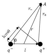
Рис. 1

Так как $lll r$, можно считать, что:

[r_–r_+approx lcostheta , r_-cdot r_+approx r^2left(3right).]

При этом местоположение точки A можно характеризовать вектором$overrightarrow{ r}$ с началом в любой точке диполя, ввиду малых геометрических размеров диполя. В таком случае формулу (2) можно записать в виде:

[varphi left(rright)=frac{1}{4pi {varepsilon }_0varepsilon }frac{overrightarrow{p_e}cdot overrightarrow{r}}{r^3}left(4right),]

где $qlcostheta =frac{overrightarrow{p_e}cdot overrightarrow{r}}{r}.$ Зная связь напряженности поля и потенциала:

[overrightarrow{E}=-gradvarphi (5)]

запишем формулу для напряженности поля диполя, которая будет иметь вид:

[overrightarrow{E}=frac{1}{4pi {varepsilon }_0varepsilon }left(frac{3left({overrightarrow{p}}_ecdot overrightarrow{r}right)overrightarrow{r}}{r^5}-frac{overrightarrow{p_e}}{r^3}right)left(6right).]

Согласно формуле (6) напряженность поля диполя убывает быстрее, чем напряженность кулоновского поля одиночного заряда, пропорционально третьей степени расстояния. Силовые линии электростатического поля около диполя изображены на рис. 2.

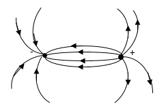
Рис. 2

Модуль вектора сопряженности

Если сферическую систему координат разместить так, чтобы ее центр совпал с серединой плеча диполя, а полярная ось была параллельна $overrightarrow{p_e}$ (рис.3), то составляющие вектора напряженности будут иметь вид:

[E_r=frac{1}{2pi {varepsilon }_0varepsilon }frac{p_ecos vartheta}{r^3},E_vartheta=frac{1}{4pi {varepsilon }_0varepsilon }frac{p_esin vartheta}{r^3},E_{varphi }=0. left(7right).]

В таком случае модуль вектора напряженности равен:

[E=frac{1}{4pi {varepsilon }_0varepsilon }frac{p_e}{r^3}sqrt{3{cos}^2vartheta+1}left(8right).]

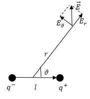
Рис. 3

Вычисление момента сил

В однородном поле сила, которая действует на диполь со стороны поля ($overrightarrow{F}$), равна нулю, так как к зарядам приложены одинаковые по модулю и противоположные по направлению силы:

[overrightarrow{F}={overrightarrow{F}}_++{overrightarrow{F}}_-=0left(9right),]

где ${overrightarrow{F}}_+$- сила, действующая на положительный заряд диполя, ${overrightarrow{F}}$ – сила, действующая на отрицательный заряд диполя.

Момент этих сил равен:

[overrightarrow{M}=overrightarrow{p_e}times overrightarrow{E}left(10right).]

Момент сил $overrightarrow{M}$ стремится повернуть ось диполя в направлении поля $overrightarrow{E}.$ Существует два положения равновесия диполя: диполь параллелен полю (устойчивое положение) и антипараллелен (неустойчивое положение).

Если поле не однородно, то сила (сумма сил действующих на положительный и отрицательный заряд) не равна нулю.$ overrightarrow{F}={overrightarrow{F}}_++{overrightarrow{F}}_-ne 0$. В этом случае сила равна:

[overrightarrow{F}=qleft({overrightarrow{E}}_+-{overrightarrow{E}}_-right)left(11right).]

В том случае, если мы имеем дело с точечным диполем (плечо диполя очень мало), то сила, действующая на диполь, может быть записана как:

[overrightarrow{F}=p_{ex}frac{partial overrightarrow{E}}{?x}+p_{ey}frac{partial overrightarrow{E}}{partial y}+p_{ez}frac{partial overrightarrow{E}}{partial z}left(12right).]

или, что то же самое, но короче:

[overrightarrow{F}=left(overrightarrow{p}overrightarrow{nabla }right)overrightarrow{E}left(13right).]

Источник

Определение[править | править код]

Дипольный момент для атома с квантовой точки зрения[править | править код]

Электрическое поле диполя[править | править код]

Действие поля на диполь[править | править код]

Единицы измерения электрического дипольного момента[править | править код]

Поляризация[править | править код]

Дипольный момент элементарных частиц[править | править код]

Дипольное приближение[править | править код]

Дипольное приближение для системы источников[править | править код]

Дипольное приближение для действия внешнего поля на систему зарядов[править | править код]

Примечания[править | править код]

Литература[править | править код]

3.1 Дипольный момент системы зарядов, поляризация диэлектриков

Теоретическая часть.

§1. Электрический диполь. Электрический дипольный момент.

§2. Диполь в однородном и неоднородном электрическом поле. Момент сил, действующий на диполь в электрическом поле.

§3. Полярные и неполярные диэлектрики.

Elementary definition[edit]

Energy and torque[edit]

Expression (general case)[edit]

Potential and field of an electric dipole[edit]

Dipole moment density and polarization density[edit]

Medium with charge and dipole densities[edit]

Surface charge[edit]

Dielectric sphere in uniform external electric field[edit]

General media[edit]

Electric dipole moments of fundamental particles[edit]

Dipole moments of molecules[edit]

See also[edit]

Notes[edit]

References[edit]

Further reading[edit]

External links[edit]

Модуль вектора сопряженности

Вычисление момента сил

Добавить комментарий Отменить ответ

Определение[править | править код]

Дипольный момент для атома с квантовой точки зрения[править | править код]

Электрическое поле диполя[править | править код]

Действие поля на диполь[править | править код]

Единицы измерения электрического дипольного момента[править | править код]

Поляризация[править | править код]

Дипольный момент элементарных частиц[править | править код]

Дипольное приближение[править | править код]

Дипольное приближение для системы источников[править | править код]

Дипольное приближение для действия внешнего поля на систему зарядов[править | править код]

Примечания[править | править код]

Литература[править | править код]

3.1 Дипольный момент системы зарядов, поляризация диэлектриков

Теоретическая часть.

§1. Электрический диполь. Электрический дипольный момент.

§2. Диполь в однородном и неоднородном электрическом поле. Момент сил, действующий на диполь в электрическом поле.

§3. Полярные и неполярные диэлектрики.

Elementary definition[edit]

Energy and torque[edit]

Expression (general case)[edit]

Potential and field of an electric dipole[edit]

Dipole moment density and polarization density[edit]

Medium with charge and dipole densities[edit]

Surface charge[edit]

Dielectric sphere in uniform external electric field[edit]

General media[edit]

Electric dipole moments of fundamental particles[edit]

Dipole moments of molecules[edit]

See also[edit]

Notes[edit]

References[edit]

Further reading[edit]

External links[edit]

Модуль вектора сопряженности

Вычисление момента сил

Вам также может понравиться

Как найти стикер в вк в магазине

Даны координаты вершин треугольника как найти высоту

Как найти силу нормального давления в физике

Добавить комментарий Отменить ответ