Как найти энтропию информатика - Сайт, где вы сможете решить свои вопросы

Теория информации

Энтропия Дифференциальная энтропия Условная энтропия Совместная энтропия Взаимная информация Условная взаимная информация Относительная энтропия Энтропийная скорость
Свойство асимптотической равнораспределенности Теория частотных искажений
Теорема Шеннона об источнике шифрования Пропускная способность Теоремы Шеннона для канала с шумами Теорема Шеннона — Хартли

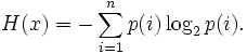
Информацио́нная энтропи́я — мера неопределённости некоторой системы (в статистической физике или теории информации), в частности, непредсказуемость появления какого-либо символа первичного алфавита. В последнем случае при отсутствии информационных потерь энтропия численно равна количеству информации на символ передаваемого сообщения.

Например, в последовательности букв, составляющих какое-либо предложение на русском языке, разные буквы появляются с разной частотностью, поэтому неопределённость появления для некоторых букв меньше, чем для других. Если же учесть, что некоторые сочетания букв (в этом случае говорят об энтропии -го порядка, см. ниже) встречаются очень редко, то неопределённость уменьшается еще сильнее.

Формальные определения[править | править код]

Информационная двоичная энтропия, при отсутствии информационных потерь, рассчитывается по формуле Хартли:

${displaystyle i=log _{2}N}$ ,

где — мощность алфавита, — количество информации в каждом символе сообщения. Для случайной величины , принимающей независимых случайных значений $x_{i}$ с вероятностями $p_{i}$ (), формула Хартли переходит в формулу Шеннона:

${displaystyle H(x)=-sum _{i=1}^{n}p_{i}log _{2}p_{i}.}$

Эта величина также называется средней энтропией сообщения. Величина ${displaystyle H_{i}=-log _{2}{p_{i}}}$ называется частной энтропией, характеризующей только -e состояние.

Таким образом, энтропия системы является суммой с противоположным знаком всех относительных частотностей появления состояния (события) с номером , умноженных на их же двоичные логарифмы^[1]. Это определение для дискретных случайных событий можно формально расширить для непрерывных распределений, заданных плотностью распределения вероятностей, однако полученный функционал будет обладать несколько иными свойствами (см. дифференциальная энтропия).

В общем случае, основание логарифма в определении энтропии может быть любым, большим 1 (так как алфавитом, состоящим только из одного символа, нельзя передавать информацию); выбор основания логарифма определяет единицу измерения энтропии. Для информационных систем, основанных на двоичной системе счисления, единицей измерения информационной энтропии (собственно, информации) является бит. В задачах математической статистики более удобным может оказаться применение натурального логарифма, в этом случае единицей измерения информационной энтропии является нат.

Определение по Шеннону[править | править код]

Клод Шеннон предположил, что прирост информации равен утраченной неопределённости, и задал требования к её измерению:

мера должна быть непрерывной; то есть изменение значения величины вероятности на малую величину должно вызывать малое результирующее изменение функции;
в случае, когда все варианты (буквы в приведённом примере) равновероятны, увеличение количества вариантов (букв) должно всегда увеличивать значение функции;
должна быть возможность сделать выбор (в нашем примере — букв) в два шага, в которых значение функции конечного результата должно являться суммой функций промежуточных результатов.^{[прояснить]}

Поэтому функция энтропии должна удовлетворять условиям

$H(p_{1},;ldots ,;p_{n})$ определена и непрерывна для всех ${displaystyle p_{1},dotsc ,p_{n}}$ , где $p_{i}in [0,;1]$ для всех и ${displaystyle p_{1}+dotsb +p_{n}=1}$ . (Эта функция зависит только от распределения вероятностей, но не от алфавита.)
Для целых положительных , должно выполняться следующее неравенство:

$Hunderbrace {left({frac {1}{n}},;ldots ,;{frac {1}{n}}right)}_{n}<Hunderbrace {left({frac {1}{n+1}},;ldots ,;{frac {1}{n+1}}right)}_{{n+1}}.$
Для целых положительных $b_{i}$ , где $b_{1}+ldots +b_{k}=n$ , должно выполняться равенство

$Hunderbrace {left({frac {1}{n}},;ldots ,;{frac {1}{n}}right)}_{n}=Hleft({frac {b_{1}}{n}},;ldots ,;{frac {b_{k}}{n}}right)+sum _{{i=1}}^{k}{frac {b_{i}}{n}}Hunderbrace {left({frac {1}{b_{i}}},;ldots ,;{frac {1}{b_{i}}}right)}_{{b_{i}}}.$

Шеннон показал,^[2] что единственная функция, удовлетворяющая этим требованиям, имеет вид

$-Ksum _{{i=1}}^{n}p(i)log _{2}p(i),$

где — положительная константа (и в действительности нужна только для выбора единицы измерения энтропии; изменение этой константы равносильно изменению основания логарифма).

Шеннон определил, что измерение энтропии ( $H=-p_{1}log _{2}p_{1}-ldots -p_{n}log _{2}p_{n}$ ), применяемое к источнику информации, может определить требования к минимальной пропускной способности канала, требуемой для надёжной передачи информации в виде закодированных двоичных чисел. Для вывода формулы Шеннона необходимо вычислить математическое ожидание «количества информации», содержащегося в цифре из источника информации. Мера энтропии Шеннона выражает неуверенность реализации случайной переменной. Таким образом, энтропия является разницей между информацией, содержащейся в сообщении, и той частью информации, которая точно известна (или хорошо предсказуема) в сообщении. Примером этого является избыточность языка — имеются явные статистические закономерности в появлении букв, пар последовательных букв, троек и т. д. (см. цепи Маркова).

Определение энтропии Шеннона связано с понятием термодинамической энтропии. Больцман и Гиббс проделали большую работу по статистической термодинамике, которая способствовала принятию слова «энтропия» в информационную теорию. Существует связь между термодинамической и информационной энтропией. Например, демон Максвелла также противопоставляет термодинамическую энтропию информации, и получение какого-либо количества информации равно потерянной энтропии.

Определение с помощью собственной информации[править | править код]

Также можно определить энтропию случайной величины, предварительно введя понятие распределения случайной величины , имеющей конечное число значений:^[3]

$P_{X}(x_{i})=p_{i},quad p_{i}geqslant 0,;i=1,;2,;ldots ,;n$

$sum _{{i=1}}^{n}p_{i}=1$

и собственной информации:

$I(X)=-log P_{X}(X).$

Тогда энтропия определяется как:

${displaystyle H(X)=mathbb {E} (I(X))=-sum _{i=1}^{n}p(i)log p(i).}$

Единицы измерения информационной энтропии[править | править код]

От основания логарифма зависит единица измерения количества информации и энтропии: бит, нат, трит или хартли.

Свойства[править | править код]

Энтропия является количеством, определённым в контексте вероятностной модели для источника данных. Например, кидание монеты имеет энтропию:

$-2left({frac {1}{2}}log _{2}{frac {1}{2}}right)=-log _{2}{frac {1}{2}}=log _{2}2=1$

бит на одно кидание (при условии его независимости), а количество возможных состояний равно: $2^{1}=2$

возможных состояния (значения) («орёл» и «решка»).

У источника, который генерирует строку, состоящую только из букв «А», энтропия равна нулю: $-sum _{{i=1}}^{infty }log _{2}1=0$ , а количество возможных состояний равно: $2^{0}=1$ возможное состояние (значение) («А») и от основания логарифма не зависит.
Это тоже информация, которую тоже надо учитывать. Примером запоминающих устройств, в которых используются разряды с энтропией, равной нулю, но с количеством информации, равным одному возможному состоянию, то есть не равным нулю, являются разряды данных записанных в ПЗУ, в которых каждый разряд имеет только одно возможное состояние.

Так, например, опытным путём можно установить, что энтропия английского текста равна 1,5 бит на символ, что будет варьироваться для разных текстов. Степень энтропии источника данных означает среднее число битов на элемент данных, требуемых для их (данных) зашифровки без потери информации, при оптимальном кодировании.

Некоторые биты данных могут не нести информации. Например, структуры данных часто хранят избыточную информацию или имеют идентичные секции независимо от информации в структуре данных.
Количество энтропии не всегда выражается целым числом битов.

Математические свойства[править | править код]

Неотрицательность: .
Ограниченность: ${displaystyle H(X)=-mathop {mathbb {E} } (log _{2}p_{i})=sum _{i=1}^{n}p_{i}log _{2}{frac {1}{p_{i}}}=sum _{i=1}^{n}p_{i}f(g_{i})leqslant fleft(sum _{i=1}^{n}p_{i}g_{i}right)=log _{2}n}$ , что вытекает из неравенства Йенсена для вогнутой функции $f(g_{i})=log _{2}g_{i}$ и $g_{i}={frac {1}{p_{i}}}$ . Если все элементов из равновероятны, $H(X)=log _{2}n$ .
Если независимы, то .
Энтропия — выпуклая вверх функция распределения вероятностей элементов.
Если имеют одинаковое распределение вероятностей элементов, то .

Эффективность[править | править код]

Алфавит может иметь вероятностное распределение, далекое от равномерного. Если исходный алфавит содержит символов, тогда его можно сравнить с «оптимизированным алфавитом», вероятностное распределение которого — равномерное. Соотношение энтропии исходного и оптимизированного алфавита — это эффективность исходного алфавита, которая может быть выражена в процентах. Эффективность исходного алфавита с символами может быть также определена как его -арная энтропия.

Энтропия ограничивает максимально возможное сжатие без потерь (или почти без потерь), которое может быть реализовано при использовании теоретически — типичного набора или, на практике, — кодирования Хаффмана, кодирования Лемпеля — Зива — Велча или арифметического кодирования.

Вариации и обобщения[править | править код]

b-арная энтропия[править | править код]

В общем случае b-арная энтропия (где b равно 2, 3, …) источника с исходным алфавитом $S={a_{1},;ldots ,;a_{n}}$ и дискретным распределением вероятности $P={p_{1},;ldots ,;p_{n}},$ где $p_{i}$ является вероятностью $a_{i}$ ( $p_{i}=p(a_{i})$ ), определяется формулой:

$H_{b}({mathcal {S}})=-sum _{{i=1}}^{n}p_{i}log _{b}p_{i}.$

В частности, при b=2 , мы получаем обычную двоичную энтропию, измеряемую в битах. При b=3 , мы получаем тринарную энтропию, измеряемую в тритах (один трит имеет источник информации с тремя равновероятными состояниями). При b=e мы получаем информацию, измеряемую в натах.

Условная энтропия[править | править код]

Если следование символов алфавита не независимо (например, во французском языке после буквы «q» почти всегда следует «u», а после слова «передовик» в советских газетах обычно следовало слово «производства» или «труда»), количество информации, которую несёт последовательность таких символов (а, следовательно, и энтропия) меньше. Для учёта таких фактов используется условная энтропия.

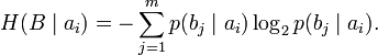
Условной энтропией первого порядка (аналогично для Марковской модели первого порядка) называется энтропия для алфавита, где известны вероятности появления одной буквы после другой (то есть вероятности двухбуквенных сочетаний):

$H_{1}({mathcal {S}})=-sum _{i}p_{i}sum _{j}p_{i}(j)log _{2}p_{i}(j),$

где — это состояние, зависящее от предшествующего символа, и $p_{i}(j)$ — это вероятность при условии, что был предыдущим символом.

Например, для русского языка без буквы «ё» $H_{0}=5,;H_{1}=4{,}358,;H_{2}=3{,}52,;H_{3}=3{,}01$ ^[4].

Через частную и общую условные энтропии полностью описываются информационные потери при передаче данных в канале с помехами. Для этого применяются так называемые канальные матрицы. Для описания потерь со стороны источника (то есть известен посланный сигнал) рассматривают условную вероятность $p(b_{j}mid a_{i})$ получения приёмником символа $b_{j}$ при условии, что был отправлен символ $a_{i}$ . При этом канальная матрица имеет следующий вид:

	$b_{1}$	$b_{2}$	…	$b_{j}$	…	$b_{m}$
$a_{1}$	$p(b_{1}mid a_{1})$	$p(b_{2}mid a_{1})$	…	$p(b_{j}mid a_{1})$	…	$p(b_{m}mid a_{1})$
$a_{2}$	$p(b_{1}mid a_{2})$	$p(b_{2}mid a_{2})$	…	$p(b_{j}mid a_{2})$	…	$p(b_{m}mid a_{2})$
…	…	…	…	…	…	…
$a_{i}$	$p(b_{1}mid a_{i})$	$p(b_{2}mid a_{i})$	…	$p(b_{j}mid a_{i})$	…	$p(b_{m}mid a_{i})$
…	…	…	…	…	…	…
	$p(b_{1}mid a_{m})$	$p(b_{2}mid a_{m})$	…	$p(b_{j}mid a_{m})$	…	$p(b_{m}mid a_{m})$

Вероятности, расположенные по диагонали, описывают вероятность правильного приёма, а сумма всех элементов любой строки даёт 1. Потери, приходящиеся на передаваемый сигнал $a_{i}$ , описываются через частную условную энтропию:

$H(Bmid a_{i})=-sum _{{j=1}}^{m}p(b_{j}mid a_{i})log _{2}p(b_{j}mid a_{i}).$

Для вычисления потерь при передаче всех сигналов используется общая условная энтропия:

$H(Bmid A)=sum _{i}p(a_{i})H(Bmid a_{i}).$

означает энтропию со стороны источника, аналогично рассматривается — энтропия со стороны приёмника: вместо $p(b_{j}mid a_{i})$ всюду указывается $p(a_{i}mid b_{j})$ (суммируя элементы строки можно получить $p(a_{i})$ , а элементы диагонали означают вероятность того, что был отправлен именно тот символ, который получен, то есть вероятность правильной передачи).

Взаимная энтропия[править | править код]

Взаимная энтропия или энтропия объединения предназначена для расчёта энтропии взаимосвязанных систем (энтропии совместного появления статистически зависимых сообщений) и обозначается H(AB) , где характеризует передатчик, а — приёмник.

Взаимосвязь переданных и полученных сигналов описывается вероятностями совместных событий $p(a_{i}b_{j})$ , и для полного описания характеристик канала требуется только одна матрица:

$p(a_{1}b_{1})$	$p(a_{1}b_{2})$	…	$p(a_{1}b_{j})$	…	$p(a_{1}b_{m})$
$p(a_{2}b_{1})$	$p(a_{2}b_{2})$	…	$p(a_{2}b_{j})$	…	$p(a_{2}b_{m})$
…	…	…	…	…	…
$p(a_{i}b_{1})$	$p(a_{i}b_{2})$	…	$p(a_{i}b_{j})$	…	$p(a_{i}b_{m})$
…	…	…	…	…	…
$p(a_{m}b_{1})$	$p(a_{m}b_{2})$	…	$p(a_{m}b_{j})$	…	$p(a_{m}b_{m})$

Для более общего случая, когда описывается не канал, а в целом взаимодействующие системы, матрица необязательно должна быть квадратной. Сумма всех элементов столбца с номером даёт $p(b_{j})$ , сумма строки с номером есть $p(a_{i})$ , а сумма всех элементов матрицы равна 1. Совместная вероятность $p(a_{i}b_{j})$ событий $a_{i}$ и $b_{j}$ вычисляется как произведение исходной и условной вероятности:

$p(a_{i}b_{j})=p(a_{i})p(b_{j}mid a_{i})=p(b_{j})p(a_{i}mid b_{j}).$

Условные вероятности производятся по формуле Байеса. Таким образом, имеются все данные для вычисления энтропий источника и приёмника:

$H(A)=-sum _{i}left(sum _{j}p(a_{i}b_{j})log sum _{j}p(a_{i}b_{j})right),$

$H(B)=-sum _{j}left(sum _{i}p(a_{i}b_{j})log sum _{i}p(a_{i}b_{j})right).$

Взаимная энтропия вычисляется последовательным суммированием по строкам (или по столбцам) всех вероятностей матрицы, умноженных на их логарифм:

$H(AB)=-sum _{i}sum _{j}p(a_{i}b_{j})log p(a_{i}b_{j}).$

Единица измерения — бит/два символа, это объясняется тем, что взаимная энтропия описывает неопределённость на пару символов: отправленного и полученного. Путём несложных преобразований также получаем

Взаимная энтропия обладает свойством информационной полноты — из неё можно получить все рассматриваемые величины.

История[править | править код]

В 1948 году, исследуя проблему рациональной передачи информации через зашумлённый коммуникационный канал, Клод Шеннон предложил революционный вероятностный подход к пониманию коммуникаций и создал первую, истинно математическую, теорию энтропии. Его сенсационные идеи быстро послужили основой разработки двух основных направлений: теории информации, которая использует понятие вероятности и эргодическую теорию для изучения статистических характеристик данных и коммуникационных систем, и теории кодирования, в которой используются главным образом алгебраические и геометрические инструменты для разработки эффективных кодов.

Понятие энтропии как меры случайности введено Шенноном в его статье «Математическая теория связи» (англ. A Mathematical Theory of Communication), опубликованной в двух частях в Bell System Technical Journal в 1948 году.

Примечания[править | править код]

↑ Данное представление удобно для работы с информацией, представленной в двоичной форме; в общем случае основание логарифма может быть другим.
↑ Shannon, Claude E. A Mathematical Theory of Communication (неопр.) // Bell System Technical Journal (англ.) (рус.. — 1948. — July (т. 27, № 3). — С. 419. — doi:10.1002/j.1538-7305.1948.tb01338.x. Архивировано 1 августа 2016 года.
↑ Габидулин Э. М., Пилипчук Н. И. Лекции по теории информации — МФТИ, 2007. — С. 16. — 214 с. — ISBN 978-5-7417-0197-3
↑ Лебедев Д. С., Гармаш В. А. О возможности увеличения скорости передачи телеграфных сообщений. — М.: Электросвязь, 1958. — № 1. — С. 68—69.

См. также[править | править код]

Дифференциальная энтропия (энтропия для непрерывного распределения)
Взаимная информация
Энтропийное кодирование
Цепь Маркова
Расстояние Кульбака — Лейблера

Ссылки[править | править код]

Shannon Claude E. A Mathematical Theory of Communication Архивная копия от 31 января 1998 на Wayback Machine (англ.)
Коротаев С. М. Энтропия и информация — универсальные естественнонаучные понятия.

Литература[править | править код]

Шеннон К. Работы по теории информации и кибернетике. — М.: Изд. иностр. лит., 2002.
Волькенштейн М. В. Энтропия и информация. — М.: Наука, 2006.
Цымбал В. П. Теория информации и кодирование. — К.: Вища Школа, 2003.
Martin, Nathaniel F.G. & England, James W. Mathematical Theory of Entropy. — Cambridge University Press, 2011. — ISBN 978-0-521-17738-2.
Шамбадаль П. Развитие и приложение понятия энтропии. — М.: Наука, 1967. — 280 с.
Мартин Н., Ингленд Дж. Математическая теория энтропии. — М.: Мир, 1988. — 350 с.
Хинчин А. Я. Понятие энтропии в теории вероятностей // Успехи математических наук. — Российская академия наук, 1953. — Т. 8, вып. 3(55). — С. 3—20.
Брюллюэн Л. Наука и теория информации. — М., 1960.
Винер Н. Кибернетика и общество. — М., 1958.
Винер Н. Кибернетика или управление и связь в животном и машине. — М., 1968.
Петрушенко Л. А. Самодвижение материи в свете кибернетики. — М., 1974.
Эшби У. Р. Введение в кибернетику. — М., 1965.
Яглом А. М., Яглом И. М. Вероятность и информация. — М., 1973.
Волькенштейн М. В. Энтропия и информация. — М.: Наука, 1986. — 192 с.
Верещагин Н.К., Щепин Е.В. Информация, кодирование и предсказание. — М.: ФМОП, МЦНМО, 2012. — 238 с. — ISBN 978-5-94057-920-5.

Источник

Формула Шеннона (Информационная энтропия)

Данная формула также как и формула Хартли, в информатике применяется для высчитывания общего количество информации при различных вероятностях.

В качестве примера различных не равных вероятностей можно привести выход людей из казармы в военной части. Из казармы могут выйти как и солдат, так и офицер, и даже генерал. Но распределение cолдатов, офицеров и генералов в казарме разное, что очевидно, ведь солдатов будет больше всего, затем по количеству идут офицеры и самый редкий вид будут генералы. Так как вероятности не равны для всех трех видов военных, для того чтобы подсчитать сколько информации займет такое событие и используется формула Шеннона.

Для других же равновероятных событий, таких как подброс монеты (вероятность того что выпадет орёл или решка будет одинаковой — 50 %) используется формула Хартли.

Интересуешься информатикой? Читайте нашу новую лекцию системы счисления

Теперь, давайте рассмотрим применение этой формулы на конкретном примере:

В каком сообщений содержится меньше всего информации (Считайте в битах):

Василий сьел 6 конфет, из них 2 было барбариски.
В комьютере 10 папок, нужный файл нашелся в 9 папке.
Баба Люда сделала 4 пирога с мясом и 4 пирога с капустой. Григорий сьел 2 пирога.
В Африке 200 дней сухая погода, а 165 дней льют муссоны. африканец охотился 40 дней в году.

В этой задаче обратим внимания что 1,2 и 3 варианты, эти варианты считать легко, так как события равновероятны. И для этого мы будем использовать формулу Хартли I = log₂N (рис.1) А вот с 4 пунком где видно, что распределение дней не равномерно(перевес в сторону сухой погоды), что же тогда нам в этом случае делать? Для таких событий и используется формула Шеннона или информационной энтропии: I = — ( p₁log₂ p₁ + p₂ log₂ p₂ + . . . + p_N log₂ p_N), (рис.3)

ФОРМУЛА КОЛИЧЕСТВА ИНФОРМАЦИИ (ФОРМУЛА ХАРТЛИ, РИС.1 )

В которой:

I — количество информации
p — вероятность того что это события случиться

Далее чтобы узнать p необходимо поделить количество интересующих нас событий на общее количество возможных вариантов.

Интересующие нас события в нашей задаче это

Было две барбариски из шести (2/6)
Была одна папка в которой нашлась нужный файл по отношению к общему количеству (1/10)
Всего пирогов было восемь из которых сьедено григорием два (2/8)
и последнее сорок дней охоты по отношению к двести засушливым дням и сорок дней охоты к сто шестидесяти пяти дождливым дням. (40/200) + (40/165)

таким образом получаем что:

ФОРМУЛА ВЕРОЯТНОСТИ ДЛЯ СОБЫТИЯ.

Где K — это интересующие нас событие, а N общее количество этих событий, также чтобы проверить себя вероятность того или иного события не может быть больше единицы. (потому что вероятных событий всегда меньше)

ФОРМУЛА ШЕННОНА ДЛЯ ПОДСЧЕТА ИНФОРМАЦИИ (РИС.3)

Вернемся к нашей задаче и посчитаем сколько информации содержится.

Кстате, при подсчёте логарифма удобно использовать сайт — https://planetcalc.ru/419/#

Для первого случая — 2/6 = 0,33 = и далее Log₂ 0,33 = 1.599 бит
Для второго случая — 1/10 = 0,10 Log₂ 0,10 = 3.322 бит
Для третьего — 2/8 = 0,25 = Log₂ 0,25 = 2 бит
Для четвертого — 40/200 + 40/165 = 0.2 и 0,24 соответственно, далее считаем по формуле -(0,2 * log₂0,2) +-(0,24 * log₂ 0.24) = 0.95856 бит

Таким образом ответ для нашей задачи получился 0.95856 бит, что значит 4 пункт.

Вот таким образом и используется формула Шеннона при подсчёте информации. Если у вас есть какие либо вопросы, или что то Вам не понятно можете задать вопросы в комментариях. (отвечаю оперативно)

Источник

Энтропия H и количество получаемой в результате снятия неопределенности информации I зависят от исходного количества рассматриваемых вариантов N и априорных вероятностей реализации каждого из них P: {p0, p1, …pN-1}, т. е. H=F(N, P). Расчет энтропии в этом случае производится по формуле Шеннона, предложенной им в 1948 году в статье «Математическая теория связи».

$H(X)= - sum_{i=1}^np(x_i)log_b p(x_i)$

Минус используется из-за того, что логарифм числа меньшего единицы, величина отрицательная. Но так как
$-log a = log frac{1}{a}$ ,
то формулу можно записать еще в виде

$H(X)= sum_{i=1}^np(x_i)log_b frac{1}{p(x_i)}$

$log_b frac{1}{p(x_i)}$
интерпретируется как частное количество информации, получаемое в случае реализации i-ого варианта ( I_i ).

Таким образом энтропия в формуле Шеннона является средней характеристикой — математическим ожиданием распределения случайной величины {I0, I1, … IN-1}, и может быть использована как мера информационной неопределенности.

Ниже два калькулятора — один рассчитывает энтропию по заданной таблице вероятностей, другой — на основе анализа встречамости символов в блоке текста.

Формула Шеннона

Точность вычисления

Знаков после запятой: 2

Формула Шеннона

Точность вычисления

Знаков после запятой: 2

Источник

In information theory, the entropy of a random variable is the average level of “information”, “surprise”, or “uncertainty” inherent to the variable’s possible outcomes. Given a discrete random variable , which takes values in the alphabet and is distributed according to :

${displaystyle mathrm {H} (X):=-sum _{xin {mathcal {X}}}p(x)log p(x)=mathbb {E} [-log p(X)],}$

where Sigma denotes the sum over the variable’s possible values. The choice of base for log , the logarithm, varies for different applications. Base 2 gives the unit of bits (or “shannons”), while base e gives “natural units” nat, and base 10 gives units of “dits”, “bans”, or “hartleys”. An equivalent definition of entropy is the expected value of the self-information of a variable.^[1]

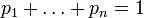
Two bits of entropy: In the case of two fair coin tosses, the information entropy in bits is the base-2 logarithm of the number of possible outcomes; with two coins there are four possible outcomes, and two bits of entropy. Generally, information entropy is the average amount of information conveyed by an event, when considering all possible outcomes.

The concept of information entropy was introduced by Claude Shannon in his 1948 paper “A Mathematical Theory of Communication”,^[2]^[3] and is also referred to as Shannon entropy. Shannon’s theory defines a data communication system composed of three elements: a source of data, a communication channel, and a receiver. The “fundamental problem of communication” – as expressed by Shannon – is for the receiver to be able to identify what data was generated by the source, based on the signal it receives through the channel.^[2]^[3] Shannon considered various ways to encode, compress, and transmit messages from a data source, and proved in his famous source coding theorem that the entropy represents an absolute mathematical limit on how well data from the source can be losslessly compressed onto a perfectly noiseless channel. Shannon strengthened this result considerably for noisy channels in his noisy-channel coding theorem.

Entropy in information theory is directly analogous to the entropy in statistical thermodynamics. The analogy results when the values of the random variable designate energies of microstates, so Gibbs formula for the entropy is formally identical to Shannon’s formula. Entropy has relevance to other areas of mathematics such as combinatorics and machine learning. The definition can be derived from a set of axioms establishing that entropy should be a measure of how informative the average outcome of a variable is. For a continuous random variable, differential entropy is analogous to entropy.

Introduction[edit]

The core idea of information theory is that the “informational value” of a communicated message depends on the degree to which the content of the message is surprising. If a highly likely event occurs, the message carries very little information. On the other hand, if a highly unlikely event occurs, the message is much more informative. For instance, the knowledge that some particular number will not be the winning number of a lottery provides very little information, because any particular chosen number will almost certainly not win. However, knowledge that a particular number will win a lottery has high informational value because it communicates the outcome of a very low probability event.

The information content, also called the surprisal or self-information, of an event is a function which increases as the probability of an event decreases. When is close to 1, the surprisal of the event is low, but if is close to 0, the surprisal of the event is high. This relationship is described by the function

${displaystyle log left({frac {1}{p(E)}}right),}$

where log is the logarithm, which gives 0 surprise when the probability of the event is 1.^[4] In fact, the log is the only function that satisfies this specific set of characterization.

Hence, we can define the information, or surprisal, of an event by

${displaystyle I(E)=-log _{2}(p(E)),}$

or equivalently,

${displaystyle I(E)=log _{2}left({frac {1}{p(E)}}right).}$

Entropy measures the expected (i.e., average) amount of information conveyed by identifying the outcome of a random trial.^[5]^: 67 This implies that casting a die has higher entropy than tossing a coin because each outcome of a die toss has smaller probability (about ) than each outcome of a coin toss ( p=1/2 ).

Consider a coin with probability p of landing on heads and probability 1 − p of landing on tails. The maximum surprise is when p = 1/2, for which one outcome is not expected over the other. In this case a coin flip has an entropy of one bit. (Similarly, one trit with equiprobable values contains $log _{2}3$ (about 1.58496) bits of information because it can have one of three values.) The minimum surprise is when p = 0 or p = 1, when the event outcome is known ahead of time, and the entropy is zero bits. When the entropy is zero bits, this is sometimes referred to as unity, where there is no uncertainty at all – no freedom of choice – no information. Other values of p give entropies between zero and one bits.

Information theory is useful to calculate the smallest amount of information required to convey a message, as in data compression. For example, consider the transmission of sequences comprising the 4 characters ‘A’, ‘B’, ‘C’, and ‘D’ over a binary channel. If all 4 letters are equally likely (25%), one can’t do better than using two bits to encode each letter. ‘A’ might code as ’00’, ‘B’ as ’01’, ‘C’ as ’10’, and ‘D’ as ’11’. However, if the probabilities of each letter are unequal, say ‘A’ occurs with 70% probability, ‘B’ with 26%, and ‘C’ and ‘D’ with 2% each, one could assign variable length codes. In this case, ‘A’ would be coded as ‘0’, ‘B’ as ’10’, ‘C’ as ‘110’, and D as ‘111’. With this representation, 70% of the time only one bit needs to be sent, 26% of the time two bits, and only 4% of the time 3 bits. On average, fewer than 2 bits are required since the entropy is lower (owing to the high prevalence of ‘A’ followed by ‘B’ – together 96% of characters). The calculation of the sum of probability-weighted log probabilities measures and captures this effect. English text, treated as a string of characters, has fairly low entropy, i.e., is fairly predictable. We can be fairly certain that, for example, ‘e’ will be far more common than ‘z’, that the combination ‘qu’ will be much more common than any other combination with a ‘q’ in it, and that the combination ‘th’ will be more common than ‘z’, ‘q’, or ‘qu’. After the first few letters one can often guess the rest of the word. English text has between 0.6 and 1.3 bits of entropy per character of the message.^[6]^: 234

Definition[edit]

Named after Boltzmann’s Η-theorem, Shannon defined the entropy Η (Greek capital letter eta) of a discrete random variable , which takes values in the alphabet and is distributed according to such that :

Here is the expected value operator, and I is the information content of X.^[7]^: 11^[8]^: 19–20
is itself a random variable.

The entropy can explicitly be written as:

${displaystyle mathrm {H} (X)=-sum _{xin {mathcal {X}}}p(x)log _{b}p(x),}$

where b is the base of the logarithm used. Common values of b are 2, Euler’s number e, and 10, and the corresponding units of entropy are the bits for b = 2, nats for b = e, and bans for b = 10.^[9]

In the case of for some , the value of the corresponding summand 0 log_b(0) is taken to be 0, which is consistent with the limit:^[10]^: 13

${displaystyle lim _{pto 0^{+}}plog(p)=0.}$

One may also define the conditional entropy of two variables and taking values from sets and respectively, as:^[10]^: 16

${displaystyle mathrm {H} (X|Y)=-sum _{x,yin {mathcal {X}}times {mathcal {Y}}}p_{X,Y}(x,y)log {frac {p_{X,Y}(x,y)}{p_{Y}(y)}},}$

where ${displaystyle p_{X,Y}(x,y):=mathbb {P} [X=x,Y=y]}$ and ${displaystyle p_{Y}(y)=mathbb {P} [Y=y]}$ . This quantity should be understood as the remaining randomness in the random variable given the random variable .

Measure theory[edit]

Entropy can be formally defined in the language of measure theory as follows:^[11] Let be a probability space. Let be an event. The surprisal of is

${displaystyle sigma _{mu }(A)=-ln mu (A).}$

The expected surprisal of is

${displaystyle h_{mu }(A)=mu (A)sigma _{mu }(A).}$

A -almost partition is a set family such that and for all distinct . (This is a relaxation of the usual conditions for a partition.) The entropy of is

${displaystyle mathrm {H} _{mu }(P)=sum _{Ain P}h_{mu }(A).}$

Let be a sigma-algebra on . The entropy of is

${displaystyle mathrm {H} _{mu }(M)=sup _{Psubseteq M}mathrm {H} _{mu }(P).}$

Finally, the entropy of the probability space is ${displaystyle mathrm {H} _{mu }(Sigma )}$ , that is, the entropy with respect to of the sigma-algebra of all measurable subsets of .

Ellerman definition[edit]

David Ellerman wanted to explain why conditional entropy and other functions had properties similar to functions in probability theory. He claims that previous definitions based on measure theory only worked with powers of 2.^[12]

Ellerman created a “logic of partitions” that is the dual of subsets of a universal set. Information is quantified as “dits” (distinctions), a measure on partitions. “Dits” can be converted into Shannon’s bits, to get the formulas for conditional entropy, etc..

Example[edit]

Entropy Η(X) (i.e. the expected surprisal) of a coin flip, measured in bits, graphed versus the bias of the coin Pr(X = 1), where X = 1 represents a result of heads.^[10]^: 14–15

Here, the entropy is at most 1 bit, and to communicate the outcome of a coin flip (2 possible values) will require an average of at most 1 bit (exactly 1 bit for a fair coin). The result of a fair die (6 possible values) would have entropy log₂6 bits.

Consider tossing a coin with known, not necessarily fair, probabilities of coming up heads or tails; this can be modelled as a Bernoulli process.

The entropy of the unknown result of the next toss of the coin is maximized if the coin is fair (that is, if heads and tails both have equal probability 1/2). This is the situation of maximum uncertainty as it is most difficult to predict the outcome of the next toss; the result of each toss of the coin delivers one full bit of information. This is because

${displaystyle {begin{aligned}mathrm {H} (X)&=-sum _{i=1}^{n}{p(x_{i})log _{b}p(x_{i})}\&=-sum _{i=1}^{2}{{frac {1}{2}}log _{2}{frac {1}{2}}}\&=-sum _{i=1}^{2}{{frac {1}{2}}cdot (-1)}=1end{aligned}}}$

However, if we know the coin is not fair, but comes up heads or tails with probabilities p and q, where p ≠ q, then there is less uncertainty. Every time it is tossed, one side is more likely to come up than the other. The reduced uncertainty is quantified in a lower entropy: on average each toss of the coin delivers less than one full bit of information. For example, if p = 0.7, then

${displaystyle {begin{aligned}mathrm {H} (X)&=-plog _{2}(p)-qlog _{2}(q)\&=-0.7log _{2}(0.7)-0.3log _{2}(0.3)\&approx -0.7cdot (-0.515)-0.3cdot (-1.737)\&=0.8816<1end{aligned}}}$

Uniform probability yields maximum uncertainty and therefore maximum entropy. Entropy, then, can only decrease from the value associated with uniform probability. The extreme case is that of a double-headed coin that never comes up tails, or a double-tailed coin that never results in a head. Then there is no uncertainty. The entropy is zero: each toss of the coin delivers no new information as the outcome of each coin toss is always certain.^[10]^: 14–15

Entropy can be normalized by dividing it by information length. This ratio is called metric entropy and is a measure of the randomness of the information.

Characterization[edit]

To understand the meaning of −Σ p_i log(p_i), first define an information function I in terms of an event i with probability p_i. The amount of information acquired due to the observation of event i follows from Shannon’s solution of the fundamental properties of information:^[13]

I(p) is monotonically decreasing in p: an increase in the probability of an event decreases the information from an observed event, and vice versa.
I(1) = 0: events that always occur do not communicate information.
I(p₁·p₂) = I(p₁) + I(p₂): the information learned from independent events is the sum of the information learned from each event.

Given two independent events, if the first event can yield one of n equiprobable outcomes and another has one of m equiprobable outcomes then there are mn equiprobable outcomes of the joint event. This means that if log₂(n) bits are needed to encode the first value and log₂(m) to encode the second, one needs log₂(mn) = log₂(m) + log₂(n) to encode both.

Shannon discovered that a suitable choice of is given by:^[14]

${displaystyle operatorname {I} (p)=log left({tfrac {1}{p}}right)=-log(p)}$

In fact, the only possible values of are for k<0 . Additionally, choosing a value for k is equivalent to choosing a value x>1 for , so that x corresponds to the base for the logarithm. Thus, entropy is characterized by the above four properties.

Proof
Let be the information function which one assumes to be twice continuously differentiable, one has: ${displaystyle {begin{aligned}&operatorname {I} (p_{1}p_{2})&= &operatorname {I} (p_{1})+operatorname {I} (p_{2})&&quad {text{Starting from property 3}}\&p_{2}operatorname {I} '(p_{1}p_{2})&= &operatorname {I} '(p_{1})&&quad {text{taking the derivative w.r.t}} p_{1}\&operatorname {I} '(p_{1}p_{2})+p_{1}p_{2}operatorname {I} ''(p_{1}p_{2})&= &0&&quad {text{taking the derivative w.r.t}} p_{2}\&operatorname {I} '(u)+uoperatorname {I} ''(u)&= &0&&quad {text{introducing}},u=p_{1}p_{2}\&(umapsto uoperatorname {I} '(u))'&= &0end{aligned}}}$ This differential equation leads to the solution for some . Property 2 gives . Property 1 and 2 give that for all , so that .

Proof

Let

be the information function which one assumes to be twice continuously differentiable, one has:

${displaystyle {begin{aligned}&operatorname {I} (p_{1}p_{2})&= &operatorname {I} (p_{1})+operatorname {I} (p_{2})&&quad {text{Starting from property 3}}\&p_{2}operatorname {I} '(p_{1}p_{2})&= &operatorname {I} '(p_{1})&&quad {text{taking the derivative w.r.t}} p_{1}\&operatorname {I} '(p_{1}p_{2})+p_{1}p_{2}operatorname {I} ''(p_{1}p_{2})&= &0&&quad {text{taking the derivative w.r.t}} p_{2}\&operatorname {I} '(u)+uoperatorname {I} ''(u)&= &0&&quad {text{introducing}},u=p_{1}p_{2}\&(umapsto uoperatorname {I} '(u))'&= &0end{aligned}}}$

This differential equation leads to the solution for some . Property 2 gives c=0 . Property 1 and 2 give that for all , so that k<0 .

The different units of information (bits for the binary logarithm log₂, nats for the natural logarithm ln, bans for the decimal logarithm log₁₀ and so on) are constant multiples of each other. For instance, in case of a fair coin toss, heads provides log₂(2) = 1 bit of information, which is approximately 0.693 nats or 0.301 decimal digits. Because of additivity, n tosses provide n bits of information, which is approximately 0.693n nats or 0.301n decimal digits.

The meaning of the events observed (the meaning of messages) does not matter in the definition of entropy. Entropy only takes into account the probability of observing a specific event, so the information it encapsulates is information about the underlying probability distribution, not the meaning of the events themselves.

Alternative characterization[edit]

Another characterization of entropy uses the following properties. We denote p_i = Pr(X = x_i) and Η_n(p₁, …, p_n) = Η(X).

Continuity: H should be continuous, so that changing the values of the probabilities by a very small amount should only change the entropy by a small amount.
Symmetry: H should be unchanged if the outcomes x_i are re-ordered. That is, ${displaystyle mathrm {H} _{n}left(p_{1},p_{2},ldots p_{n}right)=mathrm {H} _{n}left(p_{i_{1}},p_{i_{2}},ldots ,p_{i_{n}}right)}$ for any permutation ${displaystyle {i_{1},...,i_{n}}}$ of .
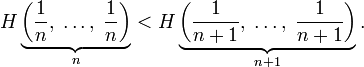
Maximum: ${displaystyle mathrm {H} _{n}}$ should be maximal if all the outcomes are equally likely i.e. ${displaystyle mathrm {H} _{n}(p_{1},ldots ,p_{n})leq mathrm {H} _{n}left({frac {1}{n}},ldots ,{frac {1}{n}}right)}$ .
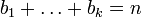
Increasing number of outcomes: for equiprobable events, the entropy should increase with the number of outcomes i.e. ${displaystyle mathrm {H} _{n}{bigg (}underbrace {{frac {1}{n}},ldots ,{frac {1}{n}}} _{n}{bigg )}<mathrm {H} _{n+1}{bigg (}underbrace {{frac {1}{n+1}},ldots ,{frac {1}{n+1}}} _{n+1}{bigg )}.}$
Additivity: given an ensemble of n uniformly distributed elements that are divided into k boxes (sub-systems) with b₁, …, b_k elements each, the entropy of the whole ensemble should be equal to the sum of the entropy of the system of boxes and the individual entropies of the boxes, each weighted with the probability of being in that particular box.

The rule of additivity has the following consequences: for positive integers b_i where b₁ + … + b_k = n,

$mathrm {H} _{n}left({frac {1}{n}},ldots ,{frac {1}{n}}right)=mathrm {H} _{k}left({frac {b_{1}}{n}},ldots ,{frac {b_{k}}{n}}right)+sum _{i=1}^{k}{frac {b_{i}}{n}},mathrm {H} _{b_{i}}left({frac {1}{b_{i}}},ldots ,{frac {1}{b_{i}}}right).$

Choosing k = n, b₁ = … = b_n = 1 this implies that the entropy of a certain outcome is zero: Η₁(1) = 0. This implies that the efficiency of a source alphabet with n symbols can be defined simply as being equal to its n-ary entropy. See also Redundancy (information theory).

Alternative characterization via additivity and subadditivity[edit]

Another succinct axiomatic characterization of Shannon entropy was given by Aczél, Forte and Ng,^[15] via the following properties:

Subadditivity: for jointly distributed random variables .
Additivity: when the random variables are independent.
Expansibility: ${displaystyle mathrm {H} _{n+1}(p_{1},ldots ,p_{n},0)=mathrm {H} _{n}(p_{1},ldots ,p_{n})}$ , i.e., adding an outcome with probability zero does not change the entropy.
Symmetry: ${displaystyle mathrm {H} _{n}(p_{1},ldots ,p_{n})}$ is invariant under permutation of .
Small for small probabilities: ${displaystyle lim _{qto 0^{+}}mathrm {H} _{2}(1-q,q)=0}$ .

It was shown that any function satisfying the above properties must be a constant multiple of Shannon entropy, with a non-negative constant.^[15] Compared to the previously mentioned characterizations of entropy, this characterization focuses on the properties of entropy as a function of random variables (subadditivity and additivity), rather than the properties of entropy as a function of the probability vector ${displaystyle p_{1},ldots ,p_{n}}$ .

It is worth noting that if we drop the “small for small probabilities” property, then must be a non-negative linear combination of the Shannon entropy and the Hartley entropy.^[15]

Further properties[edit]

The Shannon entropy satisfies the following properties, for some of which it is useful to interpret entropy as the expected amount of information learned (or uncertainty eliminated) by revealing the value of a random variable X:

Adding or removing an event with probability zero does not contribute to the entropy:

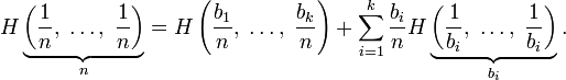
$mathrm {H} _{n+1}(p_{1},ldots ,p_{n},0)=mathrm {H} _{n}(p_{1},ldots ,p_{n})$

It can be confirmed using the Jensen inequality and then Sedrakyan’s inequality that

${displaystyle mathrm {H} (X)=mathbb {E} [-log _{b}p(X)]leq -log _{b}left(mathbb {E} [p(X)]right)leq log _{b}n}$

.^[10]^: 29

This maximal entropy of log_b(n) is effectively attained by a source alphabet having a uniform probability distribution: uncertainty is maximal when all possible events are equiprobable.

The entropy or the amount of information revealed by evaluating (X,Y) (that is, evaluating X and Y simultaneously) is equal to the information revealed by conducting two consecutive experiments: first evaluating the value of Y, then revealing the value of X given that you know the value of Y. This may be written as:^[10]^: 16

mathrm {H} (X,Y)=mathrm {H} (X|Y)+mathrm {H} (Y)=mathrm {H} (Y|X)+mathrm {H} (X).

mathrm {H} (X)+mathrm {H} (f(X)|X)=mathrm {H} (f(X))+mathrm {H} (X|f(X)),

{displaystyle mathrm {H} (f(X))leq mathrm {H} (X)}

, the entropy of a variable can only decrease when the latter is passed through a function.

If X and Y are two independent random variables, then knowing the value of Y doesn’t influence our knowledge of the value of X (since the two don’t influence each other by independence):

More generally, for any random variables X and Y, we have

{displaystyle mathrm {H} (X|Y)leq mathrm {H} (X)}

.^[10]^: 29

${displaystyle mathrm {H} (lambda p_{1}+(1-lambda )p_{2})geq lambda mathrm {H} (p_{1})+(1-lambda )mathrm {H} (p_{2})}$

for all probability mass functions ${displaystyle p_{1},p_{2}}$

and

.^[10]^: 32

Accordingly, the negative entropy (negentropy) function is convex, and its convex conjugate is LogSumExp.

Aspects[edit]

Relationship to thermodynamic entropy[edit]

The inspiration for adopting the word entropy in information theory came from the close resemblance between Shannon’s formula and very similar known formulae from statistical mechanics.

In statistical thermodynamics the most general formula for the thermodynamic entropy S of a thermodynamic system is the Gibbs entropy,

${displaystyle S=-k_{text{B}}sum p_{i}ln p_{i},}$

where k_B is the Boltzmann constant, and p_i is the probability of a microstate. The Gibbs entropy was defined by J. Willard Gibbs in 1878 after earlier work by Boltzmann (1872).^[16]

The Gibbs entropy translates over almost unchanged into the world of quantum physics to give the von Neumann entropy, introduced by John von Neumann in 1927,

${displaystyle S=-k_{text{B}},{rm {Tr}}(rho ln rho ),}$

where ρ is the density matrix of the quantum mechanical system and Tr is the trace.^[17]

At an everyday practical level, the links between information entropy and thermodynamic entropy are not evident. Physicists and chemists are apt to be more interested in changes in entropy as a system spontaneously evolves away from its initial conditions, in accordance with the second law of thermodynamics, rather than an unchanging probability distribution. As the minuteness of the Boltzmann constant k_B indicates, the changes in S / k_B for even tiny amounts of substances in chemical and physical processes represent amounts of entropy that are extremely large compared to anything in data compression or signal processing. In classical thermodynamics, entropy is defined in terms of macroscopic measurements and makes no reference to any probability distribution, which is central to the definition of information entropy.

The connection between thermodynamics and what is now known as information theory was first made by Ludwig Boltzmann and expressed by his famous equation:

${displaystyle S=k_{text{B}}ln W}$

where is the thermodynamic entropy of a particular macrostate (defined by thermodynamic parameters such as temperature, volume, energy, etc.), W is the number of microstates (various combinations of particles in various energy states) that can yield the given macrostate, and k_B is the Boltzmann constant.^[18] It is assumed that each microstate is equally likely, so that the probability of a given microstate is p_i = 1/W. When these probabilities are substituted into the above expression for the Gibbs entropy (or equivalently k_B times the Shannon entropy), Boltzmann’s equation results. In information theoretic terms, the information entropy of a system is the amount of “missing” information needed to determine a microstate, given the macrostate.

In the view of Jaynes (1957),^[19] thermodynamic entropy, as explained by statistical mechanics, should be seen as an application of Shannon’s information theory: the thermodynamic entropy is interpreted as being proportional to the amount of further Shannon information needed to define the detailed microscopic state of the system, that remains uncommunicated by a description solely in terms of the macroscopic variables of classical thermodynamics, with the constant of proportionality being just the Boltzmann constant. Adding heat to a system increases its thermodynamic entropy because it increases the number of possible microscopic states of the system that are consistent with the measurable values of its macroscopic variables, making any complete state description longer. (See article: maximum entropy thermodynamics). Maxwell’s demon can (hypothetically) reduce the thermodynamic entropy of a system by using information about the states of individual molecules; but, as Landauer (from 1961) and co-workers^[20] have shown, to function the demon himself must increase thermodynamic entropy in the process, by at least the amount of Shannon information he proposes to first acquire and store; and so the total thermodynamic entropy does not decrease (which resolves the paradox). Landauer’s principle imposes a lower bound on the amount of heat a computer must generate to process a given amount of information, though modern computers are far less efficient.

Data compression[edit]

Shannon’s definition of entropy, when applied to an information source, can determine the minimum channel capacity required to reliably transmit the source as encoded binary digits. Shannon’s entropy measures the information contained in a message as opposed to the portion of the message that is determined (or predictable). Examples of the latter include redundancy in language structure or statistical properties relating to the occurrence frequencies of letter or word pairs, triplets etc. The minimum channel capacity can be realized in theory by using the typical set or in practice using Huffman, Lempel–Ziv or arithmetic coding. (See also Kolmogorov complexity.) In practice, compression algorithms deliberately include some judicious redundancy in the form of checksums to protect against errors. The entropy rate of a data source is the average number of bits per symbol needed to encode it. Shannon’s experiments with human predictors show an information rate between 0.6 and 1.3 bits per character in English;^[21] the PPM compression algorithm can achieve a compression ratio of 1.5 bits per character in English text.

If a compression scheme is lossless – one in which you can always recover the entire original message by decompression – then a compressed message has the same quantity of information as the original but communicated in fewer characters. It has more information (higher entropy) per character. A compressed message has less redundancy. Shannon’s source coding theorem states a lossless compression scheme cannot compress messages, on average, to have more than one bit of information per bit of message, but that any value less than one bit of information per bit of message can be attained by employing a suitable coding scheme. The entropy of a message per bit multiplied by the length of that message is a measure of how much total information the message contains. Shannon’s theorem also implies that no lossless compression scheme can shorten all messages. If some messages come out shorter, at least one must come out longer due to the pigeonhole principle. In practical use, this is generally not a problem, because one is usually only interested in compressing certain types of messages, such as a document in English, as opposed to gibberish text, or digital photographs rather than noise, and it is unimportant if a compression algorithm makes some unlikely or uninteresting sequences larger.

A 2011 study in Science estimates the world’s technological capacity to store and communicate optimally compressed information normalized on the most effective compression algorithms available in the year 2007, therefore estimating the entropy of the technologically available sources.^[22]^: 60–65

All figures in entropically compressed exabytes

Type of Information	1986	2007
Storage	2.6	295
Broadcast	432	1900
Telecommunications	0.281	65

The authors estimate humankind technological capacity to store information (fully entropically compressed) in 1986 and again in 2007. They break the information into three categories—to store information on a medium, to receive information through one-way broadcast networks, or to exchange information through two-way telecommunication networks.^[22]

Entropy as a measure of diversity[edit]

Entropy is one of several ways to measure biodiversity, and is applied in the form of the Shannon index.^[23] A diversity index is a quantitative statistical measure of how many different types exist in a dataset, such as species in a community, accounting for ecological richness, evenness, and dominance. Specifically, Shannon entropy is the logarithm of ¹D, the true diversity index with parameter equal to 1. The Shannon index is related to the proportional abundances of types.

Limitations of entropy[edit]

There are a number of entropy-related concepts that mathematically quantify information content in some way:

the self-information of an individual message or symbol taken from a given probability distribution,
the entropy of a given probability distribution of messages or symbols, and
the entropy rate of a stochastic process.

(The “rate of self-information” can also be defined for a particular sequence of messages or symbols generated by a given stochastic process: this will always be equal to the entropy rate in the case of a stationary process.) Other quantities of information are also used to compare or relate different sources of information.

It is important not to confuse the above concepts. Often it is only clear from context which one is meant. For example, when someone says that the “entropy” of the English language is about 1 bit per character, they are actually modeling the English language as a stochastic process and talking about its entropy rate. Shannon himself used the term in this way.

If very large blocks are used, the estimate of per-character entropy rate may become artificially low because the probability distribution of the sequence is not known exactly; it is only an estimate. If one considers the text of every book ever published as a sequence, with each symbol being the text of a complete book, and if there are N published books, and each book is only published once, the estimate of the probability of each book is 1/N, and the entropy (in bits) is −log₂(1/N) = log₂(N). As a practical code, this corresponds to assigning each book a unique identifier and using it in place of the text of the book whenever one wants to refer to the book. This is enormously useful for talking about books, but it is not so useful for characterizing the information content of an individual book, or of language in general: it is not possible to reconstruct the book from its identifier without knowing the probability distribution, that is, the complete text of all the books. The key idea is that the complexity of the probabilistic model must be considered. Kolmogorov complexity is a theoretical generalization of this idea that allows the consideration of the information content of a sequence independent of any particular probability model; it considers the shortest program for a universal computer that outputs the sequence. A code that achieves the entropy rate of a sequence for a given model, plus the codebook (i.e. the probabilistic model), is one such program, but it may not be the shortest.

The Fibonacci sequence is 1, 1, 2, 3, 5, 8, 13, …. treating the sequence as a message and each number as a symbol, there are almost as many symbols as there are characters in the message, giving an entropy of approximately log₂(n). The first 128 symbols of the Fibonacci sequence has an entropy of approximately 7 bits/symbol, but the sequence can be expressed using a formula [F(n) = F(n−1) + F(n−2) for n = 3, 4, 5, …, F(1) =1, F(2) = 1] and this formula has a much lower entropy and applies to any length of the Fibonacci sequence.

Limitations of entropy in cryptography[edit]

In cryptanalysis, entropy is often roughly used as a measure of the unpredictability of a cryptographic key, though its real uncertainty is unmeasurable. For example, a 128-bit key that is uniformly and randomly generated has 128 bits of entropy. It also takes (on average) ${displaystyle 2^{127}}$ guesses to break by brute force. Entropy fails to capture the number of guesses required if the possible keys are not chosen uniformly.^[24]^[25] Instead, a measure called guesswork can be used to measure the effort required for a brute force attack.^[26]

Other problems may arise from non-uniform distributions used in cryptography. For example, a 1,000,000-digit binary one-time pad using exclusive or. If the pad has 1,000,000 bits of entropy, it is perfect. If the pad has 999,999 bits of entropy, evenly distributed (each individual bit of the pad having 0.999999 bits of entropy) it may provide good security. But if the pad has 999,999 bits of entropy, where the first bit is fixed and the remaining 999,999 bits are perfectly random, the first bit of the ciphertext will not be encrypted at all.

Data as a Markov process[edit]

A common way to define entropy for text is based on the Markov model of text. For an order-0 source (each character is selected independent of the last characters), the binary entropy is:

${displaystyle mathrm {H} ({mathcal {S}})=-sum p_{i}log p_{i},}$

where p_i is the probability of i. For a first-order Markov source (one in which the probability of selecting a character is dependent only on the immediately preceding character), the entropy rate is:

${displaystyle mathrm {H} ({mathcal {S}})=-sum _{i}p_{i}sum _{j} p_{i}(j)log p_{i}(j),}$

^{[citation needed]}

where i is a state (certain preceding characters) and $p_{i}(j)$ is the probability of j given i as the previous character.

For a second order Markov source, the entropy rate is

${displaystyle mathrm {H} ({mathcal {S}})=-sum _{i}p_{i}sum _{j}p_{i}(j)sum _{k}p_{i,j}(k) log p_{i,j}(k).}$

Efficiency (normalized entropy)[edit]

A source alphabet with non-uniform distribution will have less entropy than if those symbols had uniform distribution (i.e. the “optimized alphabet”). This deficiency in entropy can be expressed as a ratio called efficiency^{[This quote needs a citation]}:

${displaystyle eta (X)={frac {H}{H_{max}}}=-sum _{i=1}^{n}{frac {p(x_{i})log _{b}(p(x_{i}))}{log _{b}(n)}}}$

Applying the basic properties of the logarithm, this quantity can also be expressed as:

${displaystyle eta (X)=-sum _{i=1}^{n}{frac {p(x_{i})log _{b}(p(x_{i}))}{log _{b}(n)}}=sum _{i=1}^{n}{frac {log _{b}(p(x_{i})^{-p(x_{i})})}{log _{b}(n)}}=sum _{i=1}^{n}log _{n}(p(x_{i})^{-p(x_{i})})=log _{n}(prod _{i=1}^{n}p(x_{i})^{-p(x_{i})})}$

Efficiency has utility in quantifying the effective use of a communication channel. This formulation is also referred to as the normalized entropy, as the entropy is divided by the maximum entropy ${log _{b}(n)}$ . Furthermore, the efficiency is indifferent to choice of (positive) base b, as indicated by the insensitivity within the final logarithm above thereto.

Entropy for continuous random variables[edit]

Differential entropy[edit]

The Shannon entropy is restricted to random variables taking discrete values. The corresponding formula for a continuous random variable with probability density function f(x) with finite or infinite support on the real line is defined by analogy, using the above form of the entropy as an expectation:^[10]^: 224

${displaystyle mathrm {H} (X)=mathbb {E} [-log f(X)]=-int _{mathbb {X} }f(x)log f(x),mathrm {d} x.}$

This is the differential entropy (or continuous entropy). A precursor of the continuous entropy h[f] is the expression for the functional Η in the H-theorem of Boltzmann.

Although the analogy between both functions is suggestive, the following question must be set: is the differential entropy a valid extension of the Shannon discrete entropy? Differential entropy lacks a number of properties that the Shannon discrete entropy has – it can even be negative – and corrections have been suggested, notably limiting density of discrete points.

To answer this question, a connection must be established between the two functions:

In order to obtain a generally finite measure as the bin size goes to zero. In the discrete case, the bin size is the (implicit) width of each of the n (finite or infinite) bins whose probabilities are denoted by p_n. As the continuous domain is generalized, the width must be made explicit.

To do this, start with a continuous function f discretized into bins of size Delta .
By the mean-value theorem there exists a value x_i in each bin such that

${displaystyle f(x_{i})Delta =int _{iDelta }^{(i+1)Delta }f(x),dx}$

the integral of the function f can be approximated (in the Riemannian sense) by

${displaystyle int _{-infty }^{infty }f(x),dx=lim _{Delta to 0}sum _{i=-infty }^{infty }f(x_{i})Delta ,}$

where this limit and “bin size goes to zero” are equivalent.

We will denote

${displaystyle mathrm {H} ^{Delta }:=-sum _{i=-infty }^{infty }f(x_{i})Delta log left(f(x_{i})Delta right)}$

and expanding the logarithm, we have

${displaystyle mathrm {H} ^{Delta }=-sum _{i=-infty }^{infty }f(x_{i})Delta log(f(x_{i}))-sum _{i=-infty }^{infty }f(x_{i})Delta log(Delta ).}$

As Δ → 0, we have

${begin{aligned}sum _{i=-infty }^{infty }f(x_{i})Delta &to int _{-infty }^{infty }f(x),dx=1\sum _{i=-infty }^{infty }f(x_{i})Delta log(f(x_{i}))&to int _{-infty }^{infty }f(x)log f(x),dx.end{aligned}}$

Note; log(Δ) → −∞ as Δ → 0, requires a special definition of the differential or continuous entropy:

$h[f]=lim _{Delta to 0}left(mathrm {H} ^{Delta }+log Delta right)=-int _{-infty }^{infty }f(x)log f(x),dx,$

which is, as said before, referred to as the differential entropy. This means that the differential entropy is not a limit of the Shannon entropy for n → ∞. Rather, it differs from the limit of the Shannon entropy by an infinite offset (see also the article on information dimension).

Limiting density of discrete points[edit]

It turns out as a result that, unlike the Shannon entropy, the differential entropy is not in general a good measure of uncertainty or information. For example, the differential entropy can be negative; also it is not invariant under continuous co-ordinate transformations. This problem may be illustrated by a change of units when x is a dimensioned variable. f(x) will then have the units of 1/x. The argument of the logarithm must be dimensionless, otherwise it is improper, so that the differential entropy as given above will be improper. If Δ is some “standard” value of x (i.e. “bin size”) and therefore has the same units, then a modified differential entropy may be written in proper form as:

${displaystyle mathrm {H} =int _{-infty }^{infty }f(x)log(f(x),Delta ),dx,}$

and the result will be the same for any choice of units for x. In fact, the limit of discrete entropy as would also include a term of , which would in general be infinite. This is expected: continuous variables would typically have infinite entropy when discretized. The limiting density of discrete points is really a measure of how much easier a distribution is to describe than a distribution that is uniform over its quantization scheme.

Relative entropy[edit]

Another useful measure of entropy that works equally well in the discrete and the continuous case is the relative entropy of a distribution. It is defined as the Kullback–Leibler divergence from the distribution to a reference measure m as follows. Assume that a probability distribution p is absolutely continuous with respect to a measure m, i.e. is of the form p(dx) = f(x)m(dx) for some non-negative m-integrable function f with m-integral 1, then the relative entropy can be defined as

$D_{mathrm {KL} }(p|m)=int log(f(x))p(dx)=int f(x)log(f(x))m(dx).$

In this form the relative entropy generalizes (up to change in sign) both the discrete entropy, where the measure m is the counting measure, and the differential entropy, where the measure m is the Lebesgue measure. If the measure m is itself a probability distribution, the relative entropy is non-negative, and zero if p = m as measures. It is defined for any measure space, hence coordinate independent and invariant under co-ordinate reparameterizations if one properly takes into account the transformation of the measure m. The relative entropy, and (implicitly) entropy and differential entropy, do depend on the “reference” measure m.

Use in combinatorics[edit]

Entropy has become a useful quantity in combinatorics.

Loomis–Whitney inequality[edit]

A simple example of this is an alternative proof of the Loomis–Whitney inequality: for every subset A ⊆ Z^d, we have

$|A|^{d-1}leq prod _{i=1}^{d}|P_{i}(A)|$

where P_i is the orthogonal projection in the ith coordinate:

$P_{i}(A)={(x_{1},ldots ,x_{i-1},x_{i+1},ldots ,x_{d}):(x_{1},ldots ,x_{d})in A}.$

The proof follows as a simple corollary of Shearer’s inequality: if X₁, …, X_d are random variables and S₁, …, S_n are subsets of {1, …, d} such that every integer between 1 and d lies in exactly r of these subsets, then

$mathrm {H} [(X_{1},ldots ,X_{d})]leq {frac {1}{r}}sum _{i=1}^{n}mathrm {H} [(X_{j})_{jin S_{i}}]$

where $(X_{j})_{jin S_{i}}$ is the Cartesian product of random variables X_j with indexes j in S_i (so the dimension of this vector is equal to the size of S_i).

We sketch how Loomis–Whitney follows from this: Indeed, let X be a uniformly distributed random variable with values in A and so that each point in A occurs with equal probability. Then (by the further properties of entropy mentioned above) Η(X) = log|A|, where |A| denotes the cardinality of A. Let S_i = {1, 2, …, i−1, i+1, …, d}. The range of $(X_{j})_{jin S_{i}}$ is contained in P_i(A) and hence $mathrm {H} [(X_{j})_{jin S_{i}}]leq log |P_{i}(A)|$ . Now use this to bound the right side of Shearer’s inequality and exponentiate the opposite sides of the resulting inequality you obtain.

Approximation to binomial coefficient[edit]

For integers 0 < k < n let q = k/n. Then

${frac {2^{nmathrm {H} (q)}}{n+1}}leq {tbinom {n}{k}}leq 2^{nmathrm {H} (q)},$

where

$mathrm {H} (q)=-qlog _{2}(q)-(1-q)log _{2}(1-q).$

^[27]^: 43

Proof (sketch)
Note that ${tbinom {n}{k}}q^{qn}(1-q)^{n-nq}$ is one term of the expression $sum _{i=0}^{n}{tbinom {n}{i}}q^{i}(1-q)^{n-i}=(q+(1-q))^{n}=1.$ Rearranging gives the upper bound. For the lower bound one first shows, using some algebra, that it is the largest term in the summation. But then, ${displaystyle {binom {n}{k}}q^{qn}(1-q)^{n-nq}geq {frac {1}{n+1}}}$ since there are n + 1 terms in the summation. Rearranging gives the lower bound.

Proof (sketch)

Note that ${tbinom {n}{k}}q^{qn}(1-q)^{n-nq}$

is one term of the expression

$sum _{i=0}^{n}{tbinom {n}{i}}q^{i}(1-q)^{n-i}=(q+(1-q))^{n}=1.$

Rearranging gives the upper bound. For the lower bound one first shows, using some algebra, that it is the largest term in the summation. But then,

${displaystyle {binom {n}{k}}q^{qn}(1-q)^{n-nq}geq {frac {1}{n+1}}}$

since there are n + 1 terms in the summation. Rearranging gives the lower bound.

A nice interpretation of this is that the number of binary strings of length n with exactly k many 1’s is approximately $2^{nmathrm {H} (k/n)}$ .^[28]

Use in machine learning[edit]

Machine learning techniques arise largely from statistics and also information theory. In general, entropy is a measure of uncertainty and the objective of machine learning is to minimize uncertainty.

Decision tree learning algorithms use relative entropy to determine the decision rules that govern the data at each node.^[29] The Information gain in decision trees , which is equal to the difference between the entropy of and the conditional entropy of given , quantifies the expected information, or the reduction in entropy, from additionally knowing the value of an attribute . The information gain is used to identify which attributes of the dataset provide the most information and should be used to split the nodes of the tree optimally.

Bayesian inference models often apply the Principle of maximum entropy to obtain Prior probability distributions.^[30] The idea is that the distribution that best represents the current state of knowledge of a system is the one with the largest entropy, and is therefore suitable to be the prior.

Classification in machine learning performed by logistic regression or artificial neural networks often employs a standard loss function, called cross entropy loss, that minimizes the average cross entropy between ground truth and predicted distributions.^[31] In general, cross entropy is a measure of the differences between two datasets similar to the KL divergence (also known as relative entropy).

References[edit]

^ Pathria, R. K.; Beale, Paul (2011). Statistical Mechanics (Third ed.). Academic Press. p. 51. ISBN 978-0123821881.
^ ^a ^b Shannon, Claude E. (July 1948). “A Mathematical Theory of Communication”. Bell System Technical Journal. 27 (3): 379–423. doi:10.1002/j.1538-7305.1948.tb01338.x. hdl:10338.dmlcz/101429. (PDF, archived from here)
^ ^a ^b Shannon, Claude E. (October 1948). “A Mathematical Theory of Communication”. Bell System Technical Journal. 27 (4): 623–656. doi:10.1002/j.1538-7305.1948.tb00917.x. hdl:11858/00-001M-0000-002C-4317-B. (PDF, archived from here)
^ “Entropy (for data science) Clearly Explained!!!”. YouTube.
^ MacKay, David J.C. (2003). Information Theory, Inference, and Learning Algorithms. Cambridge University Press. ISBN 0-521-64298-1.
^ Schneier, B: Applied Cryptography, Second edition, John Wiley and Sons.
^ Borda, Monica (2011). Fundamentals in Information Theory and Coding. Springer. ISBN 978-3-642-20346-6.
^ Han, Te Sun; Kobayashi, Kingo (2002). Mathematics of Information and Coding. American Mathematical Society. ISBN 978-0-8218-4256-0.
^ Schneider, T.D, Information theory primer with an appendix on logarithms, National Cancer Institute, 14 April 2007.
^ ^a ^b ^c ^d ^e ^f ^g ^h ⁱ ^j ^k Thomas M. Cover; Joy A. Thomas (1991). Elements of Information Theory. Hoboken, New Jersey: Wiley. ISBN 978-0-471-24195-9.
^ Entropy at the nLab
^ Ellerman, David (October 2017). “Logical Information Theory: New Logical Foundations for Information Theory” (PDF). Logic Journal of the IGPL. 25 (5): 806–835. doi:10.1093/jigpal/jzx022. Retrieved 2 November 2022.
^ Carter, Tom (March 2014). An introduction to information theory and entropy (PDF). Santa Fe. Retrieved 4 August 2017.
^ Chakrabarti, C. G., and Indranil Chakrabarty. “Shannon entropy: axiomatic characterization and application.” International Journal of Mathematics and Mathematical Sciences 2005.17 (2005): 2847-2854 url
^ ^a ^b ^c Aczél, J.; Forte, B.; Ng, C. T. (1974). “Why the Shannon and Hartley entropies are ‘natural’“. Advances in Applied Probability. 6 (1): 131-146. doi:10.2307/1426210. JSTOR 1426210. S2CID 204177762.
^ Compare: Boltzmann, Ludwig (1896, 1898). Vorlesungen über Gastheorie : 2 Volumes – Leipzig 1895/98 UB: O 5262-6. English version: Lectures on gas theory. Translated by Stephen G. Brush (1964) Berkeley: University of California Press; (1995) New York: Dover ISBN 0-486-68455-5
^ Życzkowski, Karol (2006). Geometry of Quantum States: An Introduction to Quantum Entanglement. Cambridge University Press. p. 301.
^ Sharp, Kim; Matschinsky, Franz (2015). “Translation of Ludwig Boltzmann’s Paper “On the Relationship between the Second Fundamental Theorem of the Mechanical Theory of Heat and Probability Calculations Regarding the Conditions for Thermal Equilibrium”“. Entropy. 17: 1971–2009. doi:10.3390/e17041971.
^ Jaynes, E. T. (15 May 1957). “Information Theory and Statistical Mechanics”. Physical Review. 106 (4): 620–630. Bibcode:1957PhRv..106..620J. doi:10.1103/PhysRev.106.620.
^ Landauer, R. (July 1961). “Irreversibility and Heat Generation in the Computing Process”. IBM Journal of Research and Development. 5 (3): 183–191. doi:10.1147/rd.53.0183. ISSN 0018-8646.
^ Mark Nelson (24 August 2006). “The Hutter Prize”. Retrieved 27 November 2008.
^ ^a ^b “The World’s Technological Capacity to Store, Communicate, and Compute Information”, Martin Hilbert and Priscila López (2011), Science, 332(6025); free access to the article through here: martinhilbert.net/WorldInfoCapacity.html
^ Spellerberg, Ian F.; Fedor, Peter J. (2003). “A tribute to Claude Shannon (1916–2001) and a plea for more rigorous use of species richness, species diversity and the ‘Shannon–Wiener’ Index”. Global Ecology and Biogeography. 12 (3): 177–179. doi:10.1046/j.1466-822X.2003.00015.x. ISSN 1466-8238.
^ Massey, James (1994). “Guessing and Entropy” (PDF). Proc. IEEE International Symposium on Information Theory. Retrieved 31 December 2013.
^ Malone, David; Sullivan, Wayne (2005). “Guesswork is not a Substitute for Entropy” (PDF). Proceedings of the Information Technology & Telecommunications Conference. Retrieved 31 December 2013.
^ Pliam, John (1999). “Selected Areas in Cryptography”. International Workshop on Selected Areas in Cryptography. Lecture Notes in Computer Science. Vol. 1758. pp. 62–77. doi:10.1007/3-540-46513-8_5. ISBN 978-3-540-67185-5.
^ Aoki, New Approaches to Macroeconomic Modeling.
^ Probability and Computing, M. Mitzenmacher and E. Upfal, Cambridge University Press
^ Batra, Mridula; Agrawal, Rashmi (2018). Panigrahi, Bijaya Ketan; Hoda, M. N.; Sharma, Vinod; Goel, Shivendra (eds.). “Comparative Analysis of Decision Tree Algorithms”. Nature Inspired Computing. Advances in Intelligent Systems and Computing. Singapore: Springer. 652: 31–36. doi:10.1007/978-981-10-6747-1_4. ISBN 978-981-10-6747-1.
^ Jaynes, Edwin T. (September 1968). “Prior Probabilities”. IEEE Transactions on Systems Science and Cybernetics. 4 (3): 227–241. doi:10.1109/TSSC.1968.300117. ISSN 2168-2887.
^ Rubinstein, Reuven Y.; Kroese, Dirk P. (9 March 2013). The Cross-Entropy Method: A Unified Approach to Combinatorial Optimization, Monte-Carlo Simulation and Machine Learning. Springer Science & Business Media. ISBN 978-1-4757-4321-0.

This article incorporates material from Shannon’s entropy on PlanetMath, which is licensed under the Creative Commons Attribution/Share-Alike License.

External links[edit]

“Entropy”, Encyclopedia of Mathematics, EMS Press, 2001 [1994]
“Entropy” at Rosetta Code—repository of implementations of Shannon entropy in different programming languages.
Entropy an interdisciplinary journal on all aspects of the entropy concept. Open access.

Источник

Информационная
энтропия

Содержание

1
Формальные определения

1.1
Определение по Шеннону
1.2
Определение с помощью собственной
информации

2
Свойства

2.1
Математические свойства
2.2
Эффективность

3
Вариации и обобщения

3.1
b-арная
энтропия
3.2
Условная энтропия
3.3
Взаимная энтропия

4
История

5
Примечания

6
См. также

7
Ссылки

8
Литература

Информацио́нная энтропи́я –
мера неопределённости
или непредсказуемости информации,
неопределённость появления какого-либо
символа первичного
алфавита. При отсутствии
информационных потерь численно равна
количеству информации на символ
передаваемого сообщения.

Например, в последовательности
букв, составляющих какое-либо предложение
на русском языке, разные буквы появляются
с разной частотой, поэтому неопределённость
появления для некоторых букв меньше,
чем для других. Если же учесть, что
некоторые сочетания букв (в этом случае
говорят об энтропии n-ого
порядка, см. ниже)
встречаются очень редко, то неопределённость
ещё более уменьшается.

Энтропия –
это количество информации, приходящейся
на одно элементарное сообщение источника,
вырабатывающего статистически независимые
сообщения.

Формальные определения

Информационная двоичная
энтропия для независимых
случайных событий x
с n
возможными состояниями (от 1 до n)
рассчитывается по формуле:

Эта величина также называется
средней энтропией
сообщения.

Величина p(i)
–
относительная
частота появления события i.

Величина

называется частной
энтропией, характеризующей
только i-e
состояние.

Таким образом, энтропия
события x
является суммой (с противоположным
знаком) всех произведений относительных
частот появления события i,
умноженных на их же двоичные логарифмы^[1].
Это определение для дискретных случайных
событий можно расширить для функции
распределения вероятностей.

Определение по Шеннону

Шеннон
предположил, что прирост
информации равен утраченной
неопределённости, и задал требования
к её измерению:

мера должна быть непрерывной; то есть
изменение значения величины вероятности
на малую величину должно вызывать малое
результирующее изменение функции;
в случае, когда все варианты (буквы в
приведённом примере) равновероятны,
увеличение количества вариантов (букв)
должно всегда увеличивать значение
функции;
должна существовать
возможность сделать выбор (в нашем
примере букв) в два шага, в которых
значение функции конечного результата
должно являться суммой функций
промежуточных результатов.

__________________________________________________________________________

Поэтому функция энтропии
H
должна удовлетворять условиям:

определена и непрерывна
для всех

,

где

для всех

и

.

(Нетрудно видеть, что эта функция зависит
только от распределения вероятностей,
но не от алфавита.)

Для целых положительных n
должно выполняться
следующее неравенство:

Для целых положительных
b_i,
где

,
должно выполняться равенство:

Шеннон
показал,^[^{источник?}^]
что единственная функция, удовлетворяющая
этим требованиям,
имеет вид:

где K в
константа (и в действительности нужна
только для выбора единиц измерения).

Шеннон
определил, что измерение энтропии (
),
применяемое к источнику информации,
может определить требования к минимальной
пропускной способности канала, требуемой
для надёжной передачи информации в виде
закодированных двоичных чисел. Для
вывода формулы Шеннона необходимо
вычислить математическое
ожидание
«количества информации», содержащегося
в цифре из источника информации. Мера
энтропии Шеннона выражает неуверенность
реализации случайной переменной. Таким
образом, энтропия является разницей
между информацией, содержащейся в
сообщении, и той частью информации,
которая точно известна (или хорошо
предсказуема) в сообщении. Примером
этого является избыточность
языка в
имеются явные статистические закономерности
в появлении букв, пар последовательных
букв, троек и т. д. (см. цепи
Маркова).

Определение
энтропии Шеннона связано с понятием
термодинамической
энтропии.
Больцман
и Гиббс
проделали большую работу по статистической
термодинамике, которая способствовала
принятию слова «энтропия» в информационную
теорию. Существует связь между
термодинамической и информационной
энтропией. Например, демон
Максвелла
также противопоставляет термодинамическую
энтропию информации, и получение
какого-либо количества информации равно
потерянной энтропии.

Определение с
помощью собственной информации

Также можно определить
энтропию случайной величины, введя
предварительно понятия распределения
случайной величины X,
имеющей конечное число значений:^[2]

и собственной
информации:

I(X)
= в logP_X(X).

Тогда энтропия определяется как:

От основания логарифма
зависит единица измерения информации
и энтропии: бит,
трит,
нат
или хартли.

Свойства

Энтропия
является количеством, определённым в
контексте вероятностной модели для
источника
данных.
Например, кидание монеты имеет энтропию
в
2 (0,5log₂0,5)
= 1
бит
на одно кидание (при условии его
независимости). У источника, который
генерирует строку, состоящую только из
букв «А», энтропия равна нулю:

.
Так, например, опытным путём можно
установить, что энтропия английского
текста равна 1,5 бит на символ, что конечно
будет варьироваться для разных текстов.
Степень энтропии источника данных
означает среднее число битов на элемент
данных, требуемых для её зашифровки без
потери информации, при оптимальном
кодировании.

Некоторые биты
данных могут не нести информации.
Например, структуры данных часто хранят
избыточную информацию, или имеют
идентичные секции независимо от
информации в структуре данных.
Количество энтропии
не всегда выражается целым числом бит.

Математические
свойства

Неотрицательность:

.
Ограниченность:

.
Равенство, если все элементы из X
равновероятны.
Если

независимы,
то

.
Энтропия в
выпуклая вверх функция распределения
вероятностей элементов.
Если

имеют
одинаковое распределение вероятностей
элементов, то H(X)
= H(Y).

Эффективность

Алфавит
может иметь вероятностное распределение
далекое от равномерного.
Если исходный алфавит содержит n
символов, тогда его можно сравнить с
«оптимизированным алфавитом»,
вероятностное распределение которого
равномерное. Соотношение энтропии
исходного и оптимизированного алфавита в
это эффективность
исходного алфавита, которая может быть
выражена в процентах. Эффективность
исходного алфавита с n
символами может быть также определена
как его n-арная
энтропия.

Энтропия
ограничивает максимально возможное
сжатие без потерь (или почти без потерь),
которое может быть реализовано при
использовании теоретически в типичного
набора
или, на практике, в кодирования
Хаффмана,
кодирования
Лемпеля в Зива в Велча
или арифметического
кодирования.

Вариации и
обобщения

b-арная
энтропия

В общем
случае b-арная
энтропия
(где b
равно 2, 3, в) источника

с
исходным
алфавитом

и
дискретным
распределением вероятности

где p_i
является вероятностью a_i
(p_i
= p(a_i)),
определяется формулой:

Условная энтропия

Если
следование символов алфавита не
независимо (например, во французском
языке
после буквы «q» почти всегда следует
«u», а после слова «передовик» в советских
газетах обычно следовало слово
«производства» или «труда»), количество
информации, которую несёт последовательность
таких символов (а, следовательно, и
энтропия), очевидно, меньше. Для учёта
таких фактов используется условная
энтропия.

Условной
энтропией
первого порядка (аналогично для Марковской
модели
первого порядка) называется энтропия
для алфавита, где известны вероятности
появления одной буквы после другой (то
есть, вероятности двухбуквенных
сочетаний):

где
i в
это состояние, зависящее от предшествующего
символа, и p_i(j) в
это вероятность j
при условии, что i
был предыдущим символом.

Например,
для русского языка без буквы «ё»

^[3].

Через
частную и общую условные энтропии
полностью описываются информационные
потери при передаче
данных
в канале с помехами. Для этого применяются
так называемые канальные
матрицы.
Для описания потерь со стороны источника
(то есть известен посланный сигнал)
рассматривают условную
вероятность

получения
приёмником символа b_j
при условии, что был отправлен символ
a_i.
При этом канальная матрица имеет
следующий вид:

	b₁	b₂	в	b_j	в	b_m
a₁			в		в
a₂			в		в
в	в	в	в	в	в	в
a_i			в		в
в	в	в	в	в	в	в
a_m			в		в

Очевидно,
вероятности, расположенные по диагонали,
описывают вероятность правильного
приёма, а сумма всех элементов столбца
даёт вероятность появления соответствующего
символа на стороне приёмника в p(b_j).
Потери, приходящиеся на передаваемый
сигнал a_i,
описываются через частную условную
энтропию:

Для вычисления
потерь при передаче всех сигналов
используется общая условная энтропия:

означает
энтропию со стороны источника, аналогично
рассматривается

в
энтропия со стороны приёмника: вместо

всюду
указывается

(суммируя
элементы строки можно получить p(a_i),
а элементы диагонали означают вероятность
того, что был отправлен именно тот
символ, который получен, то есть
вероятность правильной передачи).

Соседние файлы в предмете [НЕСОРТИРОВАННОЕ]

Источник

Формальные определения[править | править код]

Определение по Шеннону[править | править код]

Определение с помощью собственной информации[править | править код]

Единицы измерения информационной энтропии[править | править код]

Свойства[править | править код]

Математические свойства[править | править код]

Эффективность[править | править код]

Вариации и обобщения[править | править код]

b-арная энтропия[править | править код]

Условная энтропия[править | править код]

Взаимная энтропия[править | править код]

История[править | править код]

Примечания[править | править код]

См. также[править | править код]

Ссылки[править | править код]

Литература[править | править код]

Формула Шеннона (Информационная энтропия)

Формула Шеннона

Формула Шеннона

Introduction[edit]

Definition[edit]

Measure theory[edit]

Ellerman definition[edit]

Example[edit]

Characterization[edit]

Alternative characterization[edit]

Alternative characterization via additivity and subadditivity[edit]

Further properties[edit]

Aspects[edit]

Relationship to thermodynamic entropy[edit]

Data compression[edit]

Entropy as a measure of diversity[edit]

Limitations of entropy[edit]

Limitations of entropy in cryptography[edit]

Data as a Markov process[edit]

Efficiency (normalized entropy)[edit]

Entropy for continuous random variables[edit]

Differential entropy[edit]

Limiting density of discrete points[edit]

Relative entropy[edit]

Use in combinatorics[edit]

Loomis–Whitney inequality[edit]

Approximation to binomial coefficient[edit]

Use in machine learning[edit]

See also[edit]

References[edit]

Further reading[edit]

Textbooks on information theory[edit]

External links[edit]

Формальные определения

Определение по Шеннону

Вам также может понравиться

Щенок боится хозяина как исправить

Как исправить рингтон

Как найти тайники гобсона

Добавить комментарий Отменить ответ