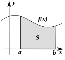
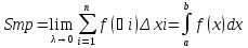
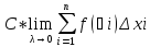
Определение интеграла было дано еще в школе при вычислении площади криволинейной трапеции. Была рассмотрена непрерывная неотрицательная функция y=f(x) на отрезке [a; b], тогда сам отрезок развивался на n равных частей точками a=x0<x1<x2<…<xn-1<xn=b. Отсюда получали, что площадь криволинейной трапеции была представлена в виде площадей элементарных треугольников
Sn=f(x0)·(x1-x0)+f(x1)·(x2-x1)+…+f(xn-1)·xn-xn-1==f(x0)·b-an+f(x1)·b-an+…+f(xn-1)·b-an==b-an·f(x0)+f(x1)+…+f(xn-1)
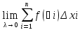
Значение данного выражения стремилось к числу I при бесконечном увеличении количества точек разбиения отрезка [a; b].
После обобщения выражения и определения получили, что любая непрерывная функция y=f(x) с числом I имеет отрезок, который и получил название определенного интеграла.
Его геометрическое понятие было показано в школе в 11 классе. Рассмотрим рисунок, приведенный ниже. Имеем изображение определенного интеграла.

В данной статье будет показано определения определенного интеграла, которые были заданы Риманом и Дарбу, Ньютоном-Лейбницом. Подробно будет показано условие интегрируемости функции на заданном определенном отрезке с перечислением интегрируемых функций.
Определенный интеграл Римана
Рассмотрим функцию y=f(x), которая определяется на заданном отрезке [a; b]. Необходимо разбить даны отрезок на n количество частей xi-1; xi, i=1, 2,…, n точками a=x0<x1<x2<…<xn-1<xn=b. Примем обозначение λ=maxi=1, 2,…, n(xi-xi-1), а сами точки xi, i=1, 2,…, n-1 необходимо выбрать таким образом, чтобы λ→0 при n→+∞. В выбранном отрезке xi-1; xi, i=1, 2,…, n необходимо выбрать точку ζi. При заданных условиях существует множество способов выбора точек xi, i=1, 2,…, n-1 и ζi, i=1, 2,…, n.
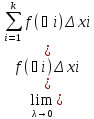
Интегральная сумма функции y=f(x) для разбиения отрезка [a; b] с выбором точек ζi, i=1, 2,…, n является выражение вида:
σ=f(ζ1)·x1-x0+f(ζ2)·x2-x1+…+f(ζn)·(xn-xn-1)==∑i=1nf(ζi)·(xi-xi-1)
Рассмотрим рисунок, приведенный ниже.

Для того, чтобы разбить заданный отрезок [a; b] и выбрать точки ζi, i=1, 2,…, n, получаем интегральную сумму. Иначе говоря, получаем множество интегральных сумм с различными вариациями выбора xi, i=1, 2,…, n и ζi, i=1, 2,…, n.
Число I называют пределом интегральных сумм σ при λ→0, когда любое малое положительное эпсилон ε>0 имеет место быть малым положительным, зависящим от эпсилон, причем δ(ε)>0, с λ<δ, тогда при выборе точек ζi, i=1, 2,…, n неравенство σ-I<ε считается справедливым.
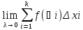
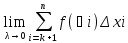
Интегрируемой на отрезке [a; b] функцией y=f(x) называют такую функцию, у которой имеется конечный предел ее интегральных сумм при λ→0. Данное значение предела называют определенным интегралом Римана.
За обозначение интеграла Римана принято брать выражение вида ∫abf(x)dx. Из определения получим, что определенный интеграл Римана записывается так: ∫abf(x)dx=limλ→0σ.
Числа a и b называют нижним и верхним пределом интегрирования, а f(x) – подынтегральная функция, где x – переменная интегрирования.
Значение определенного интеграла Римана не зависит от переменной интегрирования , тогда получаем интеграл вида ∫abf(x)dx=∫abf(t)dt=∫abf(u)du=∫abf(q)dq.
Определенный интеграл Дарбу
Чтобы понять необходимо и достаточное условие существования определенного интеграла Дарбу, необходимо применить несколько определений.
Возьмем на рассмотрение функцию y=f(x), определенную на отрезке [a; b]. Необходимо разбить заданный отрезок на n количество частей при помощи точек a=x0<x1<x2<…<xn-1<xn<b с условием λ→0 при n→+∞. Тогда mi и Mi являются нижней и верхней гранью множества значений заданной функции на i-ом отрезке i=1, 2,…, n. Получаем, что для непрерывной и ограниченной функции mi=minx∈xi-1; xif(x), Mi=maxx∈xi-1; xif(x), i=1, 2,…, n.
Полученные выражения
s=m1·(x1-x0)+m2·(x2-x1)+…+mn·(xn-xn-1)==∑i=1nmi·(xi-xi-1)
и
S=M1·(x1-x0)+M2·(x2-x1)+…+Mn·(xn-xn-1)==∑i=1nMi·(xi-xi-1)
для разбиения отрезка [a; b] называют нижней и верхней суммами Дарбу.
Рассмотрим рисунок, приведенный ниже.

Отсюда видно, для того, чтобы разбиение данного отрезка было фиксированным, необходимо использовать двойное неравенство s≤σ≤S, которое является справедливым. Иначе говоря, s и S считаются нижней и верхней гранями множества интегральных сумм.
Интегрируемость функции y=f(x) на отрезке [a; b] должна иметь достаточное условие, которое дает предел разности верхней и нижней сумм Дарбу равным нулю при λ→0, тогда условие limλ→0(S-s)=0 выполняется. Это и есть необходимое и достаточное условие существования определенного интеграла Дарбу, который так и получил название определенный интеграл Дарбу. Его обозначение записывается в виде ∫abf(x)dx.
Определенный интеграл Ньютона-Лейбница
Рассмотрим подробно понятие определенного интеграла Ньютона-Лейбница.
Если функция вида y=f(x) имеет первообразную F(x), определенную на отрезке [a; b], со значением первообразной в точке х=а равняется нулю, то есть F(a)=0. Определенный интеграл Ньютона-Лейбница – значение первообразной в точке интегрирования b, тогда получаем выражение вида ∫abf(x)dx=F(b) при F(a)=0.
Данное определение связано в формулой Ньютона-Лейбница ∫abf(x)dx=F(b)-F(a). В ней F(x) является первообразной из множества, а определенный интеграл имеет первообразную, которая становится равной нулю при х=а.
Необходимое условие интегрируемости функции на отрезке, виды интегрируемых функций
Рассмотрим необходимое условие существования определенного интеграла функции на отрезке.
Когда функция вида y=f(x) интегрируема на отрезке [a; b], то имеется в виду, что она им ограничена. Условие считается необходимым, но не достаточным, так как функция ограничена отрезком, при этом она не всегда на нем интегрируема. Это условие применяют для проверки возможности интегрирования имеющейся функции на заданном отрезке. Иначе говоря, проверяется ее ограниченность.
Виды функций, для которых существует определенный интеграл:
- когда функция непрерывна на отрезке [a; b], значит интегрируема;
- когда функция ограничена на отрезке [a; b] и непрерывна в точках, кроме конечного числа, тогда считается, что она интегрируема на отрезке [a; b].
Рассмотрим рисунок, приведенный ниже. На нем располагается пример интегрируемой функции.

Итоги
Задавание определенного интеграла Римана происходит через предел интегральных сумм, а интеграл Дарбу – предел разности верхних и нижних сумм Дарбу, в свою очередь интеграл Ньютона-Лейбница – при помощи значения первообразной.
Одновременное существование интеграла Римана и Ньютона-Лейбница, определенных на отрезке [a; b], возможно, при этом их значения будут равными. Для ограниченной функции существование определенного интеграла Дарбу и Римана невозможно.

Геометрический смысл интеграла Римана
Интегра́л Ри́мана — наиболее широко используемый вид определённого интеграла. Очень часто под термином «определённый интеграл» понимается именно интеграл Римана, и он изучается самым первым из всех определённых интегралов во всех курсах математического анализа.[1] Введён Бернхардом Риманом в 1854 году, и является одной из первых формализаций понятия интеграла.[2]
Неформальное описание[править | править код]

Риманова сумма (суммарная площадь прямоугольников) в пределе, при измельчении разбиения, дает площадь подграфика.
Интеграл Римана есть формализация понятия площади под графиком. Разобьём отрезок, над которым мы ищем площадь, на конечное число подотрезков. На каждом из подотрезков выберем некоторую точку графика и построим вертикальный прямоугольник с подотрезком в качестве основания до той самой точки графика. Рассмотрим фигуру, полученную из таких прямоугольников. Площадь S такой фигуры при конкретном разбиении на отрезки длинами  будет задаваться суммой:

Интуитивно понятно, что если мы будем уменьшать длины этих подотрезков, то площадь такой фигуры будет всё больше и больше приближаться к площади под графиком. Именно это замечание и приводит к определению интеграла Римана.[3]
Определение[править | править код]
Классическое определение[править | править код]
Пусть на отрезке ![[a,b]](https://wikimedia.org/api/rest_v1/media/math/render/svg/9c4b788fc5c637e26ee98b45f89a5c08c85f7935) определена вещественнозначная функция
определена вещественнозначная функция  . Будем считать
  .
.
Для определения интеграла прежде всего необходимо сначала определить понятие разбиения отрезка и остальные связанные с ним определения.
Разбиением (неразмеченным) отрезка назовём конечное множество точек отрезка , в которое входят точки  и
и  . Как видно из определения, в разбиение всегда входят хотя бы две точки. Точки разбиения можно расположить по возрастанию:
  . Множество всех разбиений отрезка
 ![[a;b]](https://wikimedia.org/api/rest_v1/media/math/render/svg/68e776d74130a8890a814c1f4e74372a9110d2f9) будем обозначать
будем обозначать ![{displaystyle T[a;b]}](https://wikimedia.org/api/rest_v1/media/math/render/svg/2bed719c6751668babe56a892a7d6c2a74d0a8aa) .
.
Точки разбиения, между которыми нет других точек разбиения, называются соседними. Отрезок, концами которого являются соседние точки разбиения, называется частичным отрезком разбиения. Такие отрезки обозначим ![{displaystyle Delta _{i}=[x_{i-1};x_{i}]}](https://wikimedia.org/api/rest_v1/media/math/render/svg/ffea29c0e3574633b2901a515003a2e3e75c9f33) . Длину частичного отрезка разбиения
. Длину частичного отрезка разбиения  обозначим за . Длина наибольшего из отрезков называется диаметром разбиения. Для разбиения
  его диаметр обозначим как
  .
.
Разметкой разбиения называется конечное упорядоченное множество  такое, что
  . Множество всех разметок разбиения будем обозначать как
  .
.
Размеченным разбиением называется упорядоченная пара  , где — неразмеченное разбиение,
  — некоторая разметка . Множество всех размеченных разбиений отрезка будем обозначать как
 ![{displaystyle T'[a;b]}](https://wikimedia.org/api/rest_v1/media/math/render/svg/58d8aebb90f5cee6d217cf9e2446a9966ecb70e6) .
.
После всех этих определений можно приступить к непосредственному определению интеграла Римана.
Пусть задано некоторое размеченное разбиение . Интегральной суммой Римана функции на размеченном разбиении называется  . Интегралом Римана будет предел этих сумм при диаметре разбиения, стремящемуся к нулю. Однако здесь есть одна тонкость: это предел от функции с отмеченными разбиениями в качестве аргументов, а не числами, и обычное понятие предела при стремлении к точке здесь неприменимо. Необходимо дать формальное описание того, что же мы имеем в виду под фразой «предел при диаметре разбиения, стремящемуся к нулю»
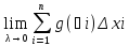
Пусть ![{displaystyle g:T'[a;b]rightarrow mathbb {R} }](https://wikimedia.org/api/rest_v1/media/math/render/svg/80cdaf43678e83c99942b127cb0be76f022cb1d7) — функция, ставящая в соответствие размеченному разбиению некоторое число. Число
— функция, ставящая в соответствие размеченному разбиению некоторое число. Число  называется пределом функции
  при диаметре разбиений, стремящемуся к нулю, если
![{displaystyle forall varepsilon >0 exists delta >0 forall (tau ,xi )in T'[a;b],d(tau )<delta :|g(tau ,xi )-c|<varepsilon }](https://wikimedia.org/api/rest_v1/media/math/render/svg/6687dc746755bf14ac95020cd306718a81587af7)
Обозначение: 
Такой предел является частным случаем предела по базе. Действительно, обозначим множество всех размеченных разбиений с диаметром меньше  как
как  . Тогда множество
  является базой на множестве , а предел, определённый выше, есть не что иное, как предел по этой базе. Таким образом, для таких пределов выполняются все свойства, присущие пределам по базе.
Наконец, мы можем дать определение интеграла Римана. Интегралом Римана функции в пределах от до называется предел интегральных сумм Римана функции на размеченных разбиениях отрезка при диаметре разбиения, стремящемуся к нулю. С использованием обозначения интеграла это записывается так:

Интеграл Римана также определяется для случая  . Для
. Для  он определяется как

Для  как
как
 [4]
[4]

Через интегралы Дарбу[править | править код]
Интеграл Римана можно определить альтернативным способом через интегралы Дарбу. Обычно такое определение доказывается как свойство, а теорема об их эквивалентности называется теоремой Дарбу. Преимущества такого определения в том, что оно позволяет обойтись без понятия размеченного разбиения, предела по разбиению и даёт более наглядный взгляд на понятие интегрируемости.
Для неразмеченного разбиения обозначим за  точную нижнюю грань функции на отрезке , за
  — точную верхнюю грань.
Нижней суммой Дарбу называется  .
.
Верхней суммой Дарбу называется  .[5]
.[5]
Нижним интегралом Дарбу называется ![{displaystyle I_{*}=sup _{tau in T[a;b]}s(f,tau )}](https://wikimedia.org/api/rest_v1/media/math/render/svg/13a4005cfd6e8efb9dc43b7c885b4345d86a7f15) .
.
Верхним интегралом Дарбу называется ![{displaystyle I^{*}=inf _{tau in T[a;b]}S(f,tau )}](https://wikimedia.org/api/rest_v1/media/math/render/svg/b1ddf6cbe9dcf31608128ecd89db5d676c538a94) .[6]
.[6]
Интегралы Дарбу существуют для любой ограниченной на отрезке интегрирования функции. Если интегралы Дарбу совпадают и конечны, то функция называется интегрируемой по Риману на отрезке , а само это число — интегралом Римана.[7]
Интеграл Дарбу может быть определён также через предел по неразмеченным разбиениям, при диаметре разбиения, стремящемуся к нулю. Предел по неразмеченным разбиениям определяется аналогично пределу по размеченным, но мы дадим формализацию и этого понятия тоже. Пусть ![{displaystyle g:T[a;b]rightarrow mathbb {R} }](https://wikimedia.org/api/rest_v1/media/math/render/svg/c79dac2484ee80d56d7c33da789bb2a8481734d1) — функция, ставящая в соответствие неразмеченному разбиению некоторое число. Число называется пределом функции при диаметре разбиений, стремящемуся к нулю, если
— функция, ставящая в соответствие неразмеченному разбиению некоторое число. Число называется пределом функции при диаметре разбиений, стремящемуся к нулю, если
![{displaystyle forall varepsilon >0 exists delta >0 forall tau in T[a;b],d(tau )<delta :|g(tau )-c|<varepsilon }](https://wikimedia.org/api/rest_v1/media/math/render/svg/6d110822413b8c2a51ada3059dbdcfe6fcd28c87)
Обозначение:  [8]
[8]
Такой предел также является частным случаем предела по базе. Базой здесь будет множество  , где
, где ![{displaystyle D_{delta }={tau in T[a;b]|d(tau )<delta }}](https://wikimedia.org/api/rest_v1/media/math/render/svg/aef8533f33bfdc88566a44982381600715833b65) .[9] Тогда:
.[9] Тогда:
Нижним интегралом Дарбу называется  .
.
Верхним интегралом Дарбу называется  .[10]
.[10]
Интегрируемые функции[править | править код]
Функция, для которой интеграл Римана в пределах от до существует (если предел равен бесконечности, то считается, что интеграл не существует), называется интегрируемой по Риману на отрезке [a;b].[11] Множество функций ![{displaystyle f:[a;b]rightarrow mathbb {R} }](https://wikimedia.org/api/rest_v1/media/math/render/svg/c50ba5f53919b297b28b62a046548c5c991b3861) , интегрируемых на отрезке , называется множеством интегрируемых на функций и обозначается
, интегрируемых на отрезке , называется множеством интегрируемых на функций и обозначается ![{displaystyle R[a;b]}](https://wikimedia.org/api/rest_v1/media/math/render/svg/abcb74d0b97873578307b5cbbec0be573e0fa637) .
.
Основным и наиболее удобным условием интегрируемости является критерий Лебега: множество интегрируемых на отрезке функций это в точности множество ограниченных и непрерывных почти всюду на этом отрезке функций. Этот критерий позволяет практически сразу получить большинство достаточных условий интегрируемости. Однако доказательство данного утверждения довольно сложное, из-за чего при методическом изложении его часто опускают и основывают дальнейшие доказательства на критерии Римана. Доказательства существования интеграла Римана на основе критерия Римана получаются сложнее, чем на основе критерия Лебега.
Критерии интегрируемости[править | править код]
- Критерий Коши. Функция интегрируема по Риману на отрезке , если
- [12]
- Данный критерий есть ни что иное, как запись критерия Коши сходимости по базе для случая интеграла Римана.
![{displaystyle forall varepsilon >0 exists delta >0 forall (tau ',xi '),(tau '',xi '')in T'[a;b],d(tau ')<delta ,d(tau '')<delta :|sigma (f,tau ',xi ')-sigma (f,tau '',xi '')|<varepsilon }](https://wikimedia.org/api/rest_v1/media/math/render/svg/d0fb1c88b7e7a4a950c6f515ede96c8badbf6f56)
- Критерий Дарбу. Функция интегрируема по Риману на отрезке , тогда и только тогда, когда верхний интеграл Дарбу совпадает с нижним и конечен.[13]
- На этом критерии основывается альтернативное определение интеграла Римана.
- Тогда -суммой функции на разбиении называется .[15][16]
- Функция интегрируема по Риману тогда и только тогда, когда она ограничена и предел -сумм при стремлении диаметра разбиения к нулю равен .[17]


- Инфинум-критерий Римана. Есть также вариация критерия Римана с использованием понятия точной грани, а не предела: функция интегрируема тогда и только тогда, когда .[18][19]
- Специальный критерий Римана. На самом деле в критерии Римана можно потребовать более слабые условия.
![{displaystyle inf _{tau in T[a;b]}Omega (f,tau )=0}](https://wikimedia.org/api/rest_v1/media/math/render/svg/3114a80c6ea453ee02e11c1dddba3a3ce80ddc70)
- Обозначим за разбиение отрезка на равных сегментов. Функция интегрируема на этом отрезке тогда и только тогда, когда последовательность стремится к нулю.[20]


- Специальный инфинум-критерий Римана. Функция интегрируема на отрезке тогда и только тогда, когда .[21]
- Критерий Дюбуа-Реймона. Определим колебание функции в точке как точную нижнюю грань значения колебаний функции в окрестности этой точки (если область определения функции не включает полную окрестность точки, то тогда рассматриваются только те точки окрестности, которые входят в область определения).

- [14]
- По сути колебание функции в точке представляет собой отличие функции от непрерывной. В точке непрерывности оно равно , в точке разрыва оно больше .
- Функция интегрируема по Риману тогда и только тогда, когда она ограничена и для любых множество всех точек в котором имеет нулевую меру Жордана (то есть для любого может быть покрыто конечным множеством интервалов с суммарной длиной меньше ).[22]


![{displaystyle xin [a;b]}](https://wikimedia.org/api/rest_v1/media/math/render/svg/6b6938dd54672227ce79bbf324f48940460dba34)


Достаточные условия интегрируемости[править | править код]
Все перечисленные далее достаточные условия интегрируемости практически сразу следуют из критерия Лебега.
Свойства[править | править код]
Дальнейшие свойства выполняются только если соответствующие интегралы существуют.
- Для существования всех этих трёх интегралов достаточно существования двух из них.
- Для любого
- [27]
- Из существования правого интеграла следует существование левого. Если , то из существования левого следует существование правого.


- Для существования всех этих трёх интегралов достаточно либо существования интеграла по большему отрезку, либо по двум меньшим.
-
- [36]

- Для существования этих двух интегралов достаточно существования левого интеграла.
- Существует вариация этого свойства на случай произвольных и .
- [37]

- Теорема о среднем. Для лучшего понимания сначала сформулируем теорему о среднем в несколько упрощённой формулировке.
- Средним значением функции на отрезке называется .
- Теорема о среднем гласит: непрерывная на отрезке функция в некоторой точке этого отрезка принимает своё среднее значение.
- Можно записать это условие без деления на , чтобы покрыть случай, когда .
- В такой записи теорема о среднем верна для любых значений и .
- На деле же верно куда более общее условие. Пусть интегрируема на , , . Тогда
- [36]
- Эту теорему также иногда называют интегральной теоремой о среднем для отличия от следующей.[38]

![{displaystyle exists cin [a;b]:f(c)={frac {1}{b-a}}int _{a}^{b}f(x),dx}](https://wikimedia.org/api/rest_v1/media/math/render/svg/e9525c5a3d3683697afa342511a0ee1a16ecef72)

![{displaystyle exists cin [a;b]:int _{a}^{b}f(x),dx=f(c)(b-a)}](https://wikimedia.org/api/rest_v1/media/math/render/svg/e6348cd5b8ef5a1db897796c809c7740cf66c351)
![{displaystyle m=inf _{xin [a;b]}f(x)}](https://wikimedia.org/api/rest_v1/media/math/render/svg/d4ab430b5fc3de238f9255677f75103904195f28)
![{displaystyle M=sup _{xin [a;b]}f(x)}](https://wikimedia.org/api/rest_v1/media/math/render/svg/eeacab1c10fbd47042d3dcc3de60f5f6e3124bb9)
![{displaystyle exists mu in [m;M]:int _{a}^{b}f(x),dx=mu (b-a)}](https://wikimedia.org/api/rest_v1/media/math/render/svg/e3d54e02f1e6d5a93dfebe94e20140a62c5af937)
-
- [39]
- Теорема вновь верна для любых и .
- Для этой теоремы можно также привести вариацию в случае непрерывности .[40]
- Иногда теоремой о среднем называют именно эту теорему, а не предыдущую. Также, для отличия от последующей, эту теорему называют первой теоремой о среднем.[41]
![{displaystyle exists mu in [m;M]:int _{a}^{b}f(x)g(x),dx=mu int _{a}^{b}g(x),dx}](https://wikimedia.org/api/rest_v1/media/math/render/svg/d2286b6177ead852590e9f446c7ae477f02aed92)
![{displaystyle exists cin [a;b]:int _{a}^{b}f(x)g(x),dx=f(c)int _{a}^{b}g(x),dx}](https://wikimedia.org/api/rest_v1/media/math/render/svg/0eb33d602d15aad6531a0d52410790017b6aa63d)
-
- [42]
- У второй теоремы о среднем есть вариации для неотрицательных функций . Пусть функция интегрируема на отрезке , а функция неотрицательна и не возрастает. Тогда
- [43]
- Пусть функция интегрируема на отрезке , а функция неотрицательна и не убывает. Тогда
- [43]
![{displaystyle exists cin [a;b]:int _{a}^{b}f(x)g(x),dx=g(a)int _{a}^{c}f(x),dx+g(b)int _{c}^{b}f(x),dx}](https://wikimedia.org/api/rest_v1/media/math/render/svg/15ce4c988fa865725bbf980da938926e660bbd8c)
![{displaystyle exists cin [a;b]:int _{a}^{b}f(x)g(x),dx=g(a)int _{a}^{c}f(x),dx}](https://wikimedia.org/api/rest_v1/media/math/render/svg/9c2a22e8953ed679df90eadc30f9beb4f352488c)
![{displaystyle exists cin [a;b]:int _{a}^{b}f(x)g(x),dx=g(b)int _{c}^{b}f(x),dx}](https://wikimedia.org/api/rest_v1/media/math/render/svg/61492c18db70ee1c547d7983c32e52bd33b43ca5)
- Независимость от множеств меры нуль. Если две функции интегрируемы на отрезке и равны на нём почти всюду, то их интегралы также равны. Таким образом, значение интеграла Римана не зависит от значения функции на множестве меры нуль. Однако его существование зависит: к примеру ноль и функция Дирихле равны почти всюду, однако интеграл от первой функции существует, а от второй нет.
Интеграл с верхним переменным пределом[править | править код]
Функция  , определяемая при помощи интеграла следующим образом

называется интегралом с верхним переменным пределом.[38]
Свойства:
Последнее свойство позволяет с помощью интеграла с верхним переменным пределом записать первообразную функции. Таким образом, оно связывает неопределённый интеграл и определённый следующим соотношением:

Это равенство также верно в случае если интегрируема и имеет первообразную на .[45]
Вычисление[править | править код]
Для вычисления интегралов Римана в простейших случаях используется формула Ньютона-Лейбница, которая является следствием свойств интеграла с верхним переменным пределом.
Формула Ньютона-Лейбница. Пусть  непрерывна на ,
  её первообразная на ,
  . Тогда
- [46]

При практическом вычислении также используют следующие приёмы:
- Замена переменной. Пусть требуется вычислить интеграл
-
- Выполняется замена , после чего пересчитываются пределы интегрирования и дифференциал:
- Тогда
- Для того, чтобы такая замена была законной, требуется непрерывность и непрерывная дифференцируемость и строгая монотонность .[47]


- Интегрирование по частям. Метод интегрирования по частям состоит в применении следующей формулы:
-
- Формула законна, если и непрерывно-дифференцируемы.[48]


На самом деле многие из указанных условий для формулы Ньютона-Лейбница и перечисленных двух приёмах избыточны и их можно существенно ослабить.[49][48][50] Однако такие условия будут более сложными, к тому же, для большинства практически встречающихся случаев указанных условий достаточно. Более того, в приведёном виде эти условия также гарантируют существование всех интегралов, что позволяет ограничиться одной лишь проверкой этих простых условий перед применением соответствующих методов.
- [51]
- [51]

- [51]

История[править | править код]
Приведенное выше определение интеграла дано Коши[52], оно применялось только для непрерывных функций.
Риман в 1854 году (опубликовано в 1868 году[2], на русском языке впервые в 1914 году[53][54]) дал это же определение без предположения непрерывности. Современный вид теории Римана придал Дарбу (1879).
Вариации и обобщения[править | править код]
- Интеграл Римана от частично заданных функций. Иногда имеет смысл определить интеграл Римана для функций, частично заданных на отрезке . Он определяется, если при любом достроении функции до полностью заданной её интеграл равен одному и тому же значению. В этом случае это значение считается интегралом Римана от частично заданной функции. К примеру: можно рассматривать функции, не определённые в конечном числе точек. Если при этом во всех остальных точках они непрерывны почти всюду, то любое достроение до полностью заданной функции интегрируемо, и их значения равны, так как значение интеграла не зависит от значения на множестве меры нуль. Для таких функций даже существует обобщение формулы Ньютона-Лейбница.[55] Однако уже даже для счётного множества это выполняется не всегда. Возьмём функцию , заданную только на множестве иррациональных чисел. Её можно разными путями доопределить до и до функции Дирихле. В одном случая она интегрируема, в другом нет. С другой стороны, если рассмотреть , неопределённый на множестве Кантора, то любое достроение такой функции будет интегрируемо.
- Интеграл Римана от векторнозначных функций. Интеграл Римана можно определить для функций, со значениями в любом топологическом векторном пространстве над . К примеру можно рассмотреть интеграл от вектор-функций (функции из со значениями в евклидовом пространстве). Такие функции интегрируются покоординатно, из-за чего практически все свойства переносятся и на них тоже.[56]
- Несобственный интеграл Римана. Иногда возникает потребность в рассмотрении интеграла на бесконечном промежутке или от неограниченной функции. Несобственный интеграл это обобщение интеграла Римана на такие случаи. Для бесконечных промежутков несобственный интеграл определяется так:

-
- Для конечных промежутков с неограниченной функцией в окрестности верхнего предела определяется так:
- Остальные случаи определяются аналогично. Если встречаются бесконечные точки разрыва внутри промежутка или оба предела бесконечны, то интеграл по аддитивности разбивается на несколько.
- Ключевая особенность такого определения в том, что для интегрируемых функций такие пределы совпадают с обычными (называемыми собственными для отличия от несобственных) интегралами. Таким образом, несобственный интеграл Римана представляет собой именно обобщение собственного.


- Кратный интеграл Римана. Кратный интеграл берётся от функций многих переменных по некоторому подмножеству . Рассматриваются разбиения этих множеств на измеримые по Жордану подмножества. В них отмечаются точки и составляются интегральные суммы (вместо длин интервалов берутся меры Жордана соответствующих подмножеств). Диаметром подмножества такого разбиения считается супремум всех расстояний между точками. Диаметром самого разбиения — минимальный диаметр разбиений подмножеств. Предел интегральных сумм при стремлении диаметра разбиений к нулю и называется кратным интегралом.
- Многие свойства кратных интегралов совпадают с обычными, но некоторые нет (к примеру, формула замены переменных). Вопреки распространённому заблуждению, точным обобщением интеграла Римана не являются, поскольку кратный интеграл берётся по неориентированному множеству, а обычный требует задания направления у отрезка.
- Криволинейный интеграл. Аналогично кратному интегралу, берётся от функции нескольких переменных, однако уже по кривой. Кривая также разбивается на подкривые, значения функции умножаются на длины соответствующих подкривых и суммируются между собой.
- Поверхностный интеграл. Практически аналогично криволинейному интегралу, с тем отличием, что берётся по поверхности, и значения функций в отмеченных точках умножаются на площади соответствующих участков.
- Интеграл Лебега. Альтернативный подход к определению интеграла. Здесь вместо разбиения области определения интегрируемой функции разбивается область значений, после чего точки разбиения умножаются на меры прообразов этих сегментов и суммируются между собой. Такие суммы при увеличении верхней точки разбиения, уменьшения нижней и стремлении его диаметра к нулю стремятся к интегралу Лебега.
См. также[править | править код]
- Интеграл Лебега и равносильные ему интеграл Даниэля, интеграл Юнга
- Интеграл Стилтьеса
- Кратный интеграл Римана
- Несобственный интеграл
Примечания[править | править код]
- ↑ Фихтенгольц, 2003, с. 107.
- ↑ 1 2 Риман (статья), 1868, с. 101-103.
- ↑ Фихтенгольц, 2003, с. 104.
- ↑ Архипов, 1999, с. 218.
- ↑ Архипов, 1999, с. 190.
- ↑ Архипов, 1999, с. 204-205.
- ↑ Архипов, 1999, с. 208.
- ↑ Ильин, 1985, с. 337.
- ↑ Архипов, 1999, с. 189.
- ↑ Ильин, 1985, с. 338.
- ↑ Архипов, 1999, с. 186-188.
- ↑ Кудрявцев, 2003, с. 539.
- ↑ Кудрявцев, 2003, с. 553.
- ↑ 1 2 3 Кудрявцев, 2003, с. 556.
- ↑ Архипов, 1999, с. 224.
- ↑ Архипов, 1999, с. 181.
- ↑ Архипов, 1999, с. 180.
- ↑ Архипов, 1999, с. 185.
- ↑ Архипов, 1999, с. 205.
- ↑ Архипов, 1999, с. 186.
- ↑ Архипов, 1999, с. 187.
- ↑ Кудрявцев, 2003, с. 563.
- ↑ Кудрявцев, 2003, с. 567.
- ↑ Кудрявцев, 2003, с. 548.
- ↑ Кудрявцев, 2003, с. 549.
- ↑ Архипов, 1999, с. 198.
- ↑ 1 2 3 4 Кудрявцев, 2003, с. 573.
- ↑ Кудрявцев, 2003, с. 574.
- ↑ 1 2 Кудрявцев, 2003, с. 578.
- ↑ Архипов, 1999, с. 203.
- ↑ Кудрявцев, 2003, с. 571.
- ↑ 1 2 Кудрявцев, 2003, с. 572.
- ↑ Архипов, 1999, с. 179.
- ↑ 1 2 Кудрявцев, 2003, с. 576.
- ↑ Кудрявцев, 2003, с. 577.
- ↑ 1 2 Фихтенгольц, 2003, с. 125.
- ↑ Кудрявцев, 2003, с. 579.
- ↑ 1 2 3 Кудрявцев, 2003, с. 587.
- ↑ Фихтенгольц, 2003, с. 126.
- ↑ Фихтенгольц, 2003, с. 127.
- ↑ Кудрявцев, 2003, с. 583.
- ↑ Фихтенгольц, 2003, с. 132.
- ↑ 1 2 Архипов, 1999, с. 215.
- ↑ Кудрявцев, 2003, с. 588.
- ↑ Кудрявцев, 2003, с. 590.
- ↑ Кудрявцев, 2003, с. 591.
- ↑ Кудрявцев, 2003, с. 596.
- ↑ 1 2 Кудрявцев, 2003, с. 600.
- ↑ Кудрявцев, 2003, с. 593.
- ↑ Кудрявцев, 2003, с. 601.
- ↑ 1 2 3 Виленкин, 1979, с. 72.
- ↑ Коши, 1831.
- ↑ Риман (книга), 1914.
- ↑ Архипов, 1999, с. 196.
- ↑ Кудрявцев, 2003, с. 595.
- ↑ Кудрявцев, 2003, с. 607.
Литература[править | править код]
- В.А. Ильин, В.А. Садовничий, Бл. Х. Сендов. Математический анализ. Начальный курс. — 2-е, переработанное. — М.: Издательство Московского Университета, 1985. — Т. 1. — 660 с.
- Фихтенгольц Г. М. Курс дифференциального и интегрального исчисления в трёх томах. — Изд. 8-е. — М.: Наука, 2003. — Т. 2. — 864 с.
- Архипов Г. И., Садовничий В. А., Чубариков В.Н. Лекции по математическому анализу / Под ред. В. А. Садовничего. — 1-е изд. — М.: Высшая школа, 1999. — 695 с. — ISBN 5-06-003596-4.
- Кудрявцев Л. Д. Курс математического анализа. В 3-х томах. Т. 1. Дифференциальное и интегральное исчисления функций одной переменной.. — М.: Дрофа, 2003. — 704 с.
- Виленкин Н.Я., Куницкая Е.С., Мордкович А.Г. Математический анализ. Интегральное исчисление. — М.: Просвящение, 1979. — 176 с.
- Cauchy A. L. Sur la mécanique céleste et sur un nouveau calcul appelé calcul des limites. — Turin, 1831.
- Riemann В. Über die Darstellbarkeit einer Function durch eine trigonometrische Reihe // Abhandlungen der Königlichen Gesellschaft der Wissenschaften zu Göttingen. — 1868. — Vol. 13. — P. 87-132.
- Риман Б. О возможности выражения функции при помощи тригонометрического ряда // Разложение функций в тригонометрические ряды / Лежен-Дирикле, Риманн, Липшиц; Пер. Г. А. Грузинцева и С. Н. Бернштейна. — Харьков: Харьковское математическое общество, 1914. — (Харьковская математическая библиотека. Серия В; № 2).
Ссылки[править | править код]
- Таблицы неопределенных и определенных интегралов — EqWorld: Мир математических уравнений.
- Строгое определение интеграла Римана.
Интеграл Римана
Определение интеграла Римана
Пусть Сумма
, где
называется интегральной суммой Римана. При этом множество точек
разбиением сегмента
а множество
— совокупностью промежуточных точек. Обозначим через
где
норму (или диаметр) разбиения
.
Число называется интегралом Римана функции
, если
Сама функция при этом называется интегрируемой по Риману на сегменте
а класс всех таких функций будем обозначать символом
Очевидно, что если
то она ограничена на этом сегменте.
Верхней и нижней интегральными суммами Дарбу ограниченной функции , соответствующими разбиению
называются соответственно суммы:
, где
Верхним и нижним интегралами Дарбу ограниченной функции называются соответственно числа:
Функция называется интегрируемой в смысле Дарбу на сегменте
если
, а общее значение верхнего и нижнего интегралов называется интегралом Дарбу функции
на сегменте
.
Теорема 1. Если интеграл Римана и определённый интеграл Ньютона-Лейбница функции существуют одновременно, то они равны друг другу.
Теорема 2. Для ограниченной функции интегралы Римана и Дарбу эквивалентны, то есть они существуют или не существуют одновременно, а в случае существования их значения совпадают.
Для интеграла Римана (Дарбу) используют то же обозначение, что и для интеграла Ньютона-Лейбница
Множество имеет лебегову (жорданову) меру 0, если
существует такое счётное (конечное) покрытие множества
семейством интегралов
, что
При этом будем писать
Теорема 3. Пусть ограниченная функция и
— множество точек разрыва. Функция
интегрируема по Риману на
тогда и только тогда, когда
— множество лебеговой меры 0.
Пусть и
. Тогда имеют место следующие свойства.
Теорема 4 (основная теорема интегрального исчисления). Функция дифференцируема в каждой точке
, в которой
непрерывна в этих точках
Теорема 5 (основная формула интегрального исчисления). Если множество точек разрыва функции = не более чем счётно, то функция
является первообразной в широком смысле для
и имеет место формула Ньютона-Лейбница
Пусть и функции
дифференцируемы на
Тогда
Пусть — дифференцируемая функция и
Тогда имеет место равенство
которое называется формулой замены переменной в интеграле Римана.
Пусть — дифференцируемые функции,
Тогда
и выполняется равенство
которое называется формулой интегрирования по частям.
Пусть . Функция
называется характеристической функцией множества
, если
Если — ограниченная функция и
то определим интеграл Римана от функции
на множестве
как
Пусть — ограниченная функция. Рассмотрим продолжение
этой функции на весь сегмент
, где
Если , то определим
Точка в упорядоченном пространстве
называется граничной точкой (точкой границы) множества
, если любая окрестность этой точки содержит как точки множества
, так и точки множества
. Совокупность всех граничных точек множества
называется границей этого множества и обозначается
.
Если граница ограниченного множество
имеет лебегову меру 0, то это множество называется измеримым по Жордану, а интеграл
называется мерой Жордана множества и обозначается
где
— произвольный сегмент, содержащий множество
.
Применение интеграла Римана
Применение интеграла Римана чаще всего проводится по одной и той же схеме, к которой приводят рассуждение геометрического или физического характера.
Функцию , где
(
– фиксированные числа из
) называют функцией промежутка, определённой на
Функция промежутка
называется аддитивной функцией промежутка (АФП), если
выполняется равенство
.
Теорема 1 (связь АФП с интегралом Римана). Если для АФП существует такая интегрируемая по Риману функция
что
выполняются соотношения
то
Эта теорема даёт возможность свести задачи вычисления площади плоской фигуры, объёма тела вращения, длины дуги кривой, статических моментов и моментов инерции кривых относительно фиксированных прямых, а также ряд других задач геометрического или физического содержания к задаче интегрирования соответствующих функций по Риману.
Поскольку применение обычного интеграла Римана (или, как ещё говорят, однократного интеграла) для вычисления различных моментов, координат центра тяжести и т.п. представляется нерациональным, то ниже приведём только схемы и методы вычисления геометрических величин, которые достаточно просто и рационально находить именно с использованием интеграла Римана.
1. Площадь криволинейной трапеции. Если функция непрерывна на отрезке
, то криволинейной трапецией
называется множество
и площадь криволинейной трапеции вычисляется по формуле
2. Площадь криволинейного сектора. Криволинейным сектором в полярной системе координат называется множество
где функция непрерывна на
.
Площадь криволинейного сектора вычисляется по формуле
3. Объём тела вращения. Если криволинейная трапеция где
, вращается вокруг оси
, то объём
образованного тела вращения вычисляется по формуле
4. Объём тела по известным поперечным сечениям. Если для некоторого тела известны площади всех его поперечных сечений вдоль некоторой числовой прямой
, которые задаются непрерывной функцией
, то объём данного тела находится по формуле
5. Длина дуги гладкой кривой. Множество называется простой гладкой кривой (траекторией), если существует отображение
где
и
При этом отображение называется параметрическим изображением кривой
, Длина
этой кривой может быть найдена по формуле
Если то последняя формула приобретает вид
Если же кривая задана в полярных координатах , то её длина вычисляется по формуле
6. Площадь криволинейной трапеции, ограниченной кривой заданной параметрически , осью абсцисс
и прямыми
и
, равна
где и
определяются из уравнений
и
при
.
7. Объем тела, полученный вращением криволинейной трапеции вокруг оси ординат
, равен
8. Объем тела, полученный вращением сектора вокруг полярной оси, равен
Математический форум (помощь с решением задач, обсуждение вопросов по математике).
Если заметили ошибку, опечатку или есть предложения, напишите в комментариях.
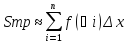
The integral as the area of a region under a curve.

A sequence of Riemann sums over a regular partition of an interval. The number on top is the total area of the rectangles, which converges to the integral of the function.

The partition does not need to be regular, as shown here. The approximation works as long as the width of each subdivision tends to zero.
In the branch of mathematics known as real analysis, the Riemann integral, created by Bernhard Riemann, was the first rigorous definition of the integral of a function on an interval. It was presented to the faculty at the University of Göttingen in 1854, but not published in a journal until 1868.[1] For many functions and practical applications, the Riemann integral can be evaluated by the fundamental theorem of calculus or approximated by numerical integration, or simulated using Monte Carlo Integration.
Overview[edit]
Let f be a non-negative real-valued function on the interval [a, b], and let S be the region of the plane under the graph of the function f and above the interval [a, b]. See the figure on the top right. This region can be expressed in set-builder notation as

We are interested in measuring the area of S. Once we have measured it, we will denote the area in the usual way by

The basic idea of the Riemann integral is to use very simple approximations for the area of S. By taking better and better approximations, we can say that “in the limit” we get exactly the area of S under the curve.
When f(x) can take negative values, the integral equals the signed area between the graph of f and the x-axis: that is, the area above the x-axis minus the area below the x-axis.
Definition[edit]
Partitions of an interval[edit]
A partition of an interval [a, b] is a finite sequence of numbers of the form

Each [xi, xi + 1] is called a sub-interval of the partition. The mesh or norm of a partition is defined to be the length of the longest sub-interval, that is,
![{displaystyle max left(x_{i+1}-x_{i}right),quad iin [0,n-1].}](https://wikimedia.org/api/rest_v1/media/math/render/svg/3c9e85d731e2ef757c1178541687891889a8d6ff)
A tagged partition P(x, t) of an interval [a, b] is a partition together with a choice of a sample point within each sub-interval: that is, numbers t0, …, tn − 1 with ti ∈ [xi, xi + 1] for each i. The mesh of a tagged partition is the same as that of an ordinary partition.
Suppose that two partitions P(x, t) and Q(y, s) are both partitions of the interval [a, b]. We say that Q(y, s) is a refinement of P(x, t) if for each integer i, with i ∈ [0, n], there exists an integer r(i) such that xi = yr(i) and such that ti = sj for some j with j ∈ [r(i), r(i + 1)]. That is, a tagged partition breaks up some of the sub-intervals and adds sample points where necessary, “refining” the accuracy of the partition.
We can turn the set of all tagged partitions into a directed set by saying that one tagged partition is greater than or equal to another if the former is a refinement of the latter.
Riemann sum[edit]
Let f be a real-valued function defined on the interval [a, b]. The Riemann sum of f with respect to the tagged partition x0, …, xn together with t0, …, tn − 1 is[2]

Each term in the sum is the product of the value of the function at a given point and the length of an interval. Consequently, each term represents the (signed) area of a rectangle with height f(ti) and width xi + 1 − xi. The Riemann sum is the (signed) area of all the rectangles.
Closely related concepts are the lower and upper Darboux sums. These are similar to Riemann sums, but the tags are replaced by the infimum and supremum (respectively) of f on each sub-interval:
![{displaystyle {begin{aligned}L(f,P)&=sum _{i=0}^{n-1}inf _{tin [x_{i},x_{i+1}]}f(t)(x_{i+1}-x_{i}),\U(f,P)&=sum _{i=0}^{n-1}sup _{tin [x_{i},x_{i+1}]}f(t)(x_{i+1}-x_{i}).end{aligned}}}](https://wikimedia.org/api/rest_v1/media/math/render/svg/9a27d85c90a22b2602c7898a1f90483f65ae2eb9)
If f is continuous, then the lower and upper Darboux sums for an untagged partition are equal to the Riemann sum for that partition, where the tags are chosen to be the minimum or maximum (respectively) of f on each subinterval. (When f is discontinuous on a subinterval, there may not be a tag that achieves the infimum or supremum on that subinterval.) The Darboux integral, which is similar to the Riemann integral but based on Darboux sums, is equivalent to the Riemann integral.
Riemann integral[edit]
Loosely speaking, the Riemann integral is the limit of the Riemann sums of a function as the partitions get finer. If the limit exists then the function is said to be integrable (or more specifically Riemann-integrable). The Riemann sum can be made as close as desired to the Riemann integral by making the partition fine enough.[3]
One important requirement is that the mesh of the partitions must become smaller and smaller, so that in the limit, it is zero. If this were not so, then we would not be getting a good approximation to the function on certain subintervals. In fact, this is enough to define an integral. To be specific, we say that the Riemann integral of f equals s if the following condition holds:
For all ε > 0, there exists δ > 0 such that for any tagged partition x0, …, xn and t0, …, tn − 1 whose mesh is less than δ, we have

Unfortunately, this definition is very difficult to use. It would help to develop an equivalent definition of the Riemann integral which is easier to work with. We develop this definition now, with a proof of equivalence following. Our new definition says that the Riemann integral of f equals s if the following condition holds:
For all ε > 0, there exists a tagged partition y0, …, ym and r0, …, rm − 1 such that for any tagged partition x0, …, xn and t0, …, tn − 1 which is a refinement of y0, …, ym and r0, …, rm − 1, we have
Both of these mean that eventually, the Riemann sum of f with respect to any partition gets trapped close to s. Since this is true no matter how close we demand the sums be trapped, we say that the Riemann sums converge to s. These definitions are actually a special case of a more general concept, a net.
As we stated earlier, these two definitions are equivalent. In other words, s works in the first definition if and only if s works in the second definition. To show that the first definition implies the second, start with an ε, and choose a δ that satisfies the condition. Choose any tagged partition whose mesh is less than δ. Its Riemann sum is within ε of s, and any refinement of this partition will also have mesh less than δ, so the Riemann sum of the refinement will also be within ε of s.
To show that the second definition implies the first, it is easiest to use the Darboux integral. First, one shows that the second definition is equivalent to the definition of the Darboux integral; for this see the Darboux Integral article. Now we will show that a Darboux integrable function satisfies the first definition. Fix ε, and choose a partition y0, …, ym such that the lower and upper Darboux sums with respect to this partition are within ε/2 of the value s of the Darboux integral. Let
![{displaystyle r=2sup _{xin [a,b]}|f(x)|.}](https://wikimedia.org/api/rest_v1/media/math/render/svg/1482a90052a248146472c490b7c64132631eb4f5)
If r = 0, then f is the zero function, which is clearly both Darboux and Riemann integrable with integral zero. Therefore, we will assume that r > 0. If m > 1, then we choose δ such that

If m = 1, then we choose δ to be less than one. Choose a tagged partition x0, …, xn and t0, …, tn − 1 with mesh smaller than δ. We must show that the Riemann sum is within ε of s.
To see this, choose an interval [xi, xi + 1]. If this interval is contained within some [yj, yj + 1], then

where mj and Mj are respectively, the infimum and the supremum of f on [yj, yj + 1]. If all intervals had this property, then this would conclude the proof, because each term in the Riemann sum would be bounded by a corresponding term in the Darboux sums, and we chose the Darboux sums to be near s. This is the case when m = 1, so the proof is finished in that case.
Therefore, we may assume that m > 1. In this case, it is possible that one of the [xi, xi + 1] is not contained in any [yj, yj + 1]. Instead, it may stretch across two of the intervals determined by y0, …, ym. (It cannot meet three intervals because δ is assumed to be smaller than the length of any one interval.) In symbols, it may happen that

(We may assume that all the inequalities are strict because otherwise we are in the previous case by our assumption on the length of δ.) This can happen at most m − 1 times.
To handle this case, we will estimate the difference between the Riemann sum and the Darboux sum by subdividing the partition x0, …, xn at yj + 1. The term f(ti)(xi + 1 − xi) in the Riemann sum splits into two terms:

Suppose, without loss of generality, that ti ∈ [yj, yj + 1]. Then

so this term is bounded by the corresponding term in the Darboux sum for yj. To bound the other term, notice that

It follows that, for some (indeed any) t*
i ∈ [yj + 1, xi + 1],

Since this happens at most m − 1 times, the distance between the Riemann sum and a Darboux sum is at most ε/2. Therefore, the distance between the Riemann sum and s is at most ε.
Examples[edit]
Let ![{displaystyle f:[0,1]to mathbb {R} }](https://wikimedia.org/api/rest_v1/media/math/render/svg/2de6d0d4c98d4ca7ad937c772dc3e3e914b062f5) be the function which takes the value 1 at every point. Any Riemann sum of f on [0, 1] will have the value 1, therefore the Riemann integral of f on [0, 1] is 1.
be the function which takes the value 1 at every point. Any Riemann sum of f on [0, 1] will have the value 1, therefore the Riemann integral of f on [0, 1] is 1.
Let ![{displaystyle I_{mathbb {Q} }:[0,1]to mathbb {R} }](https://wikimedia.org/api/rest_v1/media/math/render/svg/42a7e51a6a147bea460364984ba2ed2351383e7b) be the indicator function of the rational numbers in [0, 1]; that is,
be the indicator function of the rational numbers in [0, 1]; that is,  takes the value 1 on rational numbers and 0 on irrational numbers. This function does not have a Riemann integral. To prove this, we will show how to construct tagged partitions whose Riemann sums get arbitrarily close to both zero and one.
To start, let x0, …, xn and t0, …, tn − 1 be a tagged partition (each ti is between xi and xi + 1). Choose ε > 0. The ti have already been chosen, and we can’t change the value of f at those points. But if we cut the partition into tiny pieces around each ti, we can minimize the effect of the ti. Then, by carefully choosing the new tags, we can make the value of the Riemann sum turn out to be within ε of either zero or one.
Our first step is to cut up the partition. There are n of the ti, and we want their total effect to be less than ε. If we confine each of them to an interval of length less than ε/n, then the contribution of each ti to the Riemann sum will be at least 0 · ε/n and at most 1 · ε/n. This makes the total sum at least zero and at most ε. So let δ be a positive number less than ε/n. If it happens that two of the ti are within δ of each other, choose δ smaller. If it happens that some ti is within δ of some xj, and ti is not equal to xj, choose δ smaller. Since there are only finitely many ti and xj, we can always choose δ sufficiently small.
Now we add two cuts to the partition for each ti. One of the cuts will be at ti − δ/2, and the other will be at ti + δ/2. If one of these leaves the interval [0, 1], then we leave it out. ti will be the tag corresponding to the subinterval
![{displaystyle left[t_{i}-{frac {delta }{2}},t_{i}+{frac {delta }{2}}right].}](https://wikimedia.org/api/rest_v1/media/math/render/svg/cc67b284d007c4784218a773a332fa2f1060580b)
If ti is directly on top of one of the xj, then we let ti be the tag for both intervals:
![{displaystyle left[t_{i}-{frac {delta }{2}},x_{j}right],quad {text{and}}quad left[x_{j},t_{i}+{frac {delta }{2}}right].}](https://wikimedia.org/api/rest_v1/media/math/render/svg/4907d7e6204e6adbbd9e56a81b27fc4a7f293161)
We still have to choose tags for the other subintervals. We will choose them in two different ways. The first way is to always choose a rational point, so that the Riemann sum is as large as possible. This will make the value of the Riemann sum at least 1 − ε. The second way is to always choose an irrational point, so that the Riemann sum is as small as possible. This will make the value of the Riemann sum at most ε.
Since we started from an arbitrary partition and ended up as close as we wanted to either zero or one, it is false to say that we are eventually trapped near some number s, so this function is not Riemann integrable. However, it is Lebesgue integrable. In the Lebesgue sense its integral is zero, since the function is zero almost everywhere. But this is a fact that is beyond the reach of the Riemann integral.
There are even worse examples. is equivalent (that is, equal almost everywhere) to a Riemann integrable function, but there are non-Riemann integrable bounded functions which are not equivalent to any Riemann integrable function. For example, let C be the Smith–Volterra–Cantor set, and let IC be its indicator function. Because C is not Jordan measurable, IC is not Riemann integrable. Moreover, no function g equivalent to IC is Riemann integrable: g, like IC, must be zero on a dense set, so as in the previous example, any Riemann sum of g has a refinement which is within ε of 0 for any positive number ε. But if the Riemann integral of g exists, then it must equal the Lebesgue integral of IC, which is 1/2. Therefore, g is not Riemann integrable.
Similar concepts[edit]
It is popular to define the Riemann integral as the Darboux integral. This is because the Darboux integral is technically simpler and because a function is Riemann-integrable if and only if it is Darboux-integrable.
Some calculus books do not use general tagged partitions, but limit themselves to specific types of tagged partitions. If the type of partition is limited too much, some non-integrable functions may appear to be integrable.
One popular restriction is the use of “left-hand” and “right-hand” Riemann sums. In a left-hand Riemann sum, ti = xi for all i, and in a right-hand Riemann sum, ti = xi + 1 for all i. Alone this restriction does not impose a problem: we can refine any partition in a way that makes it a left-hand or right-hand sum by subdividing it at each ti. In more formal language, the set of all left-hand Riemann sums and the set of all right-hand Riemann sums is cofinal in the set of all tagged partitions.
Another popular restriction is the use of regular subdivisions of an interval. For example, the nth regular subdivision of [0, 1] consists of the intervals
![{displaystyle left[0,{frac {1}{n}}right],left[{frac {1}{n}},{frac {2}{n}}right],ldots ,left[{frac {n-1}{n}},1right].}](https://wikimedia.org/api/rest_v1/media/math/render/svg/70c59997a2a5eaf7cad7dec83e2d4c758c5c8309)
Again, alone this restriction does not impose a problem, but the reasoning required to see this fact is more difficult than in the case of left-hand and right-hand Riemann sums.
However, combining these restrictions, so that one uses only left-hand or right-hand Riemann sums on regularly divided intervals, is dangerous. If a function is known in advance to be Riemann integrable, then this technique will give the correct value of the integral. But under these conditions the indicator function will appear to be integrable on [0, 1] with integral equal to one: Every endpoint of every subinterval will be a rational number, so the function will always be evaluated at rational numbers, and hence it will appear to always equal one. The problem with this definition becomes apparent when we try to split the integral into two pieces. The following equation ought to hold:

If we use regular subdivisions and left-hand or right-hand Riemann sums, then the two terms on the left are equal to zero, since every endpoint except 0 and 1 will be irrational, but as we have seen the term on the right will equal 1.
As defined above, the Riemann integral avoids this problem by refusing to integrate  The Lebesgue integral is defined in such a way that all these integrals are 0.
Properties[edit]
Linearity[edit]
The Riemann integral is a linear transformation; that is, if f and g are Riemann-integrable on [a, b] and α and β are constants, then

Because the Riemann integral of a function is a number, this makes the Riemann integral a linear functional on the vector space of Riemann-integrable functions.
Integrability[edit]
A bounded function on a compact interval [a, b] is Riemann integrable if and only if it is continuous almost everywhere (the set of its points of discontinuity has measure zero, in the sense of Lebesgue measure). This is the Lebesgue-Vitali theorem (of characterization of the Riemann integrable functions). It has been proven independently by Giuseppe Vitali and by Henri Lebesgue in 1907, and uses the notion of measure zero, but makes use of neither Lebesgue’s general measure or integral.
The integrability condition can be proven in various ways,[4][5][6][7] one of which is sketched below.
| Proof |
|---|
| The proof is easiest using the Darboux integral definition of integrability (formally, the Riemann condition for integrability) – a function is Riemann integrable if and only if the upper and lower sums can be made arbitrarily close by choosing an appropriate partition.
One direction can be proven using the oscillation definition of continuity:[8] For every positive ε, Let Xε be the set of points in [a, b] with oscillation of at least ε. Since every point where f is discontinuous has a positive oscillation and vice versa, the set of points in [a, b], where f is discontinuous is equal to the union over {X1/n} for all natural numbers n. If this set does not have zero Lebesgue measure, then by countable additivity of the measure there is at least one such n so that X1/n does not have a zero measure. Thus there is some positive number c such that every countable collection of open intervals covering X1/n has a total length of at least c. In particular this is also true for every such finite collection of intervals. This remains true also for X1/n less a finite number of points (as a finite number of points can always be covered by a finite collection of intervals with arbitrarily small total length). For every partition of [a, b], consider the set of intervals whose interiors include points from X1/n. These interiors consist of a finite open cover of X1/n, possibly up to a finite number of points (which may fall on interval edges). Thus these intervals have a total length of at least c. Since in these points f has oscillation of at least 1/n, the infimum and supremum of f in each of these intervals differ by at least 1/n. Thus the upper and lower sums of f differ by at least c/n. Since this is true for every partition, f is not Riemann integrable. We now prove the converse direction using the sets Xε defined above.[9] For every ε, Xε is compact, as it is bounded (by a and b) and closed:
Now, suppose that f is continuous almost everywhere. Then for every ε, Xε has zero Lebesgue measure. Therefore, there is a countable collections of open intervals in [a, b] which is an open cover of Xε, such that the sum over all their lengths is arbitrarily small. Since Xε is compact, there is a finite subcover – a finite collections of open intervals in [a, b] with arbitrarily small total length that together contain all points in Xε. We denote these intervals {I(ε)i}, for 1 ≤ i ≤ k, for some natural k. The complement of the union of these intervals is itself a union of a finite number of intervals, which we denote {J(ε)i} (for 1 ≤ i ≤ k − 1 and possibly for i = k, k + 1 as well). We now show that for every ε > 0, there are upper and lower sums whose difference is less than ε, from which Riemann integrability follows. To this end, we construct a partition of [a, b] as follows: Denote ε1 = ε / 2(b − a) and ε2 = ε / 2(M − m), where m and M are the infimum and supremum of f on [a, b]. Since we may choose intervals {I(ε1)i} with arbitrarily small total length, we choose them to have total length smaller than ε2. Each of the intervals {J(ε1)i} has an empty intersection with Xε1, so each point in it has a neighborhood with oscillation smaller than ε1. These neighborhoods consist of an open cover of the interval, and since the interval is compact there is a finite subcover of them. This subcover is a finite collection of open intervals, which are subintervals of J(ε1)i (except for those that include an edge point, for which we only take their intersection with J(ε1)i). We take the edge points of the subintervals for all J(ε1)i − s, including the edge points of the intervals themselves, as our partition. Thus the partition divides [a, b] to two kinds of intervals:
In total, the difference between the upper and lower sums of the partition is smaller than ε, as required. |
In particular, any set that is at most countable has Lebesgue measure zero, and thus a bounded function (on a compact interval) with only finitely or countably many discontinuities is Riemann integrable. Another sufficient criterion to Riemann integrability over [a, b], but which does not involve the concept of measure, is the existence of a right-hand (or left-hand) limit at every point in [a, b) (or (a, b]).[10]
An indicator function of a bounded set is Riemann-integrable if and only if the set is Jordan measurable. The Riemann integral can be interpreted measure-theoretically as the integral with respect to the Jordan measure.
If a real-valued function is monotone on the interval [a, b] it is Riemann integrable, since its set of discontinuities is at most countable, and therefore of Lebesgue measure zero. If a real-valued function on [a, b] is Riemann integrable, it is Lebesgue integrable. That is, Riemann-integrability is a stronger (meaning more difficult to satisfy) condition than Lebesgue-integrability. The converse does not hold; not all Lebesgue-integrable functions are Riemann integrable.
The Lebesgue–Vitali theorem does not imply that all type of discontinuities have the same weight on the obstruction that a real-valued bounded function be Riemann integrable on [a, b]. In fact, certain discontinuities have absolutely no role on the Riemann integrability of the function—a consequence of the classification of the discontinuities of a function.[citation needed]
If fn is a uniformly convergent sequence on [a, b] with limit f, then Riemann integrability of all fn implies Riemann integrability of f, and

However, the Lebesgue monotone convergence theorem (on a monotone pointwise limit) does not hold for Riemann integrals. Thus, in Riemann integration, taking limits under the integral sign is far more difficult to logically justify than in Lebesgue integration.[11]
Generalizations[edit]
It is easy to extend the Riemann integral to functions with values in the Euclidean vector space  for any n. The integral is defined component-wise; in other words, if f = (f1, …, fn) then

In particular, since the complex numbers are a real vector space, this allows the integration of complex valued functions.
The Riemann integral is only defined on bounded intervals, and it does not extend well to unbounded intervals. The simplest possible extension is to define such an integral as a limit, in other words, as an improper integral:

This definition carries with it some subtleties, such as the fact that it is not always equivalent to compute the Cauchy principal value

For example, consider the sign function f(x) = sgn(x) which is 0 at x = 0, 1 for x > 0, and −1 for x < 0. By symmetry,

always, regardless of a. But there are many ways for the interval of integration to expand to fill the real line, and other ways can produce different results; in other words, the multivariate limit does not always exist. We can compute

In general, this improper Riemann integral is undefined. Even standardizing a way for the interval to approach the real line does not work because it leads to disturbingly counterintuitive results. If we agree (for instance) that the improper integral should always be

then the integral of the translation f(x − 1) is −2, so this definition is not invariant under shifts, a highly undesirable property. In fact, not only does this function not have an improper Riemann integral, its Lebesgue integral is also undefined (it equals ∞ − ∞).
Unfortunately, the improper Riemann integral is not powerful enough. The most severe problem is that there are no widely applicable theorems for commuting improper Riemann integrals with limits of functions. In applications such as Fourier series it is important to be able to approximate the integral of a function using integrals of approximations to the function. For proper Riemann integrals, a standard theorem states that if fn is a sequence of functions that converge uniformly to f on a compact set [a, b], then

On non-compact intervals such as the real line, this is false. For example, take fn(x) to be n−1 on [0, n] and zero elsewhere. For all n we have:

The sequence (fn) converges uniformly to the zero function, and clearly the integral of the zero function is zero. Consequently,

This demonstrates that for integrals on unbounded intervals, uniform convergence of a function is not strong enough to allow passing a limit through an integral sign. This makes the Riemann integral unworkable in applications (even though the Riemann integral assigns both sides the correct value), because there is no other general criterion for exchanging a limit and a Riemann integral, and without such a criterion it is difficult to approximate integrals by approximating their integrands.
A better route is to abandon the Riemann integral for the Lebesgue integral. The definition of the Lebesgue integral is not obviously a generalization of the Riemann integral, but it is not hard to prove that every Riemann-integrable function is Lebesgue-integrable and that the values of the two integrals agree whenever they are both defined. Moreover, a function f defined on a bounded interval is Riemann-integrable if and only if it is bounded and the set of points where f is discontinuous has Lebesgue measure zero.
An integral which is in fact a direct generalization of the Riemann integral is the Henstock–Kurzweil integral.
Another way of generalizing the Riemann integral is to replace the factors xk + 1 − xk in the definition of a Riemann sum by something else; roughly speaking, this gives the interval of integration a different notion of length. This is the approach taken by the Riemann–Stieltjes integral.
In multivariable calculus, the Riemann integrals for functions from  are multiple integrals.
Comparison with other theories of integration[edit]
The Riemann integral is unsuitable for many theoretical purposes. Some of the technical deficiencies in Riemann integration can be remedied with the Riemann–Stieltjes integral, and most disappear with the Lebesgue integral, though the latter does not have a satisfactory treatment of improper integrals. The gauge integral is a generalisation of the Lebesgue integral that is at once closer to the Riemann integral.
These more general theories allow for the integration of more “jagged” or “highly oscillating” functions whose Riemann integral does not exist; but the theories give the same value as the Riemann integral when it does exist.
In educational settings, the Darboux integral offers a simpler definition that is easier to work with; it can be used to introduce the Riemann integral. The Darboux integral is defined whenever the Riemann integral is, and always gives the same result. Conversely, the gauge integral is a simple but more powerful generalization of the Riemann integral and has led some educators to advocate that it should replace the Riemann integral in introductory calculus courses.[12]
See also[edit]
- Area
- Antiderivative
- Lebesgue integration
Notes[edit]
- ^ The Riemann integral was introduced in Bernhard Riemann’s paper “Über die Darstellbarkeit einer Function durch eine trigonometrische Reihe” (On the representability of a function by a trigonometric series; i.e., when can a function be represented by a trigonometric series). This paper was submitted to the University of Göttingen in 1854 as Riemann’s Habilitationsschrift (qualification to become an instructor). It was published in 1868 in Abhandlungen der Königlichen Gesellschaft der Wissenschaften zu Göttingen (Proceedings of the Royal Philosophical Society at Göttingen), vol. 13, pages 87-132. (Available online here.) For Riemann’s definition of his integral, see section 4, “Über den Begriff eines bestimmten Integrals und den Umfang seiner Gültigkeit” (On the concept of a definite integral and the extent of its validity), pages 101–103.
- ^ Krantz, Steven G. (2005). Real Analysis and Foundations. Boca Raton, Fla.: Chapman & Hall/CRC. p. 173. ISBN 1-58488-483-5. OCLC 56214595.
- ^ Taylor, Michael E. (2006). Measure Theory and Integration. American Mathematical Society. p. 1. ISBN 9780821872468.
- ^ Apostol 1974, pp. 169–172
- ^ Brown, A. B. (September 1936). “A Proof of the Lebesgue Condition for Riemann Integrability”. The American Mathematical Monthly. 43 (7): 396–398. doi:10.2307/2301737. ISSN 0002-9890. JSTOR 2301737.
- ^ Basic real analysis, by Houshang H. Sohrab, section 7.3, Sets of Measure Zero and Lebesgue’s Integrability Condition, pp. 264–271
- ^ Introduction to Real Analysis, updated April 2010, William F. Trench, 3.5 “A More Advanced Look at the Existence of the Proper Riemann Integral”, pp. 171–177
- ^ Lebesgue’s Condition, John Armstrong, December 15, 2009, The Unapologetic Mathematician
- ^ Jordan Content Integrability Condition, John Armstrong, December 9, 2009, The Unapologetic Mathematician
- ^ Metzler, R. C. (1971). “On Riemann Integrability”. The American Mathematical Monthly. 78 (10): 1129–1131. doi:10.2307/2316325. ISSN 0002-9890. JSTOR 2316325.
- ^ Cunningham, Frederick Jr. (1967). “Taking limits under the integral sign”. Mathematics Magazine. 40 (4): 179–186. doi:10.2307/2688673. JSTOR 2688673.
- ^ “An Open Letter to Authors of Calculus Books”. Retrieved 27 February 2014.
References[edit]
- Shilov, G. E., and Gurevich, B. L., 1978. Integral, Measure, and Derivative: A Unified Approach, Richard A. Silverman, trans. Dover Publications. ISBN 0-486-63519-8.
- Apostol, Tom (1974), Mathematical Analysis, Addison-Wesley
External links[edit]
 Media related to Riemann integral at Wikimedia Commons
- “Riemann integral”, Encyclopedia of Mathematics, EMS Press, 2001 [1994]
Геометрический
смысл интеграла Римана.
Определение
интеграла Римана. Функции, интегрируемые
по Риману.
Пусть
на отрезке [a,b]
задана непрер. ф-я f(x).
Разобьем отрезок на n
частей точками a=x0<x1<x2<…<xi<…<xn=b
и обозначим Δxi=xi-xi-1(i=1,2,
…,n)-
длина элементар. отрезка.
Λ=max{Δx1,Δx2,
…,Δxn}
– диаметр разбиения.
Выберем
в каждом элементарном отрезке произвольную
точку Ѯiϵ[xi-1,
xi]
(i=1,2,…,n).
Значения
ф-и в произвольной точке Ѯi
умножаем
на длину соответствующего отрезка и
суммируем по всем отрезкам. В результате
получаем выражение In= ,
,
которая назыв. интегральной суммой для
ф-иf(x)
на [a,b].
Опред.:
если существует предел интегральных
сумм при стремлении диаметра разбиения
к нулю, не зависящий от способа разбиения
отрезка [a,b]
и от выбора произвольных точек (Ѯi),
то он назыв. определенным интегралом
или интегралом Римана для ф-и f(x)
на [a,b]
и обозначается
 ,
,
при этом границы отрезка [a,b]
назыв. соответственно нижним и верхним
пределами интегрирования.
Ǝ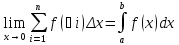 .
.
Если
для ф-и f(x)
на [a,b]
существует определенный интеграл, то
ф-ю f(x)
назыв. интегрируемой по Риману на
отрезке [a,b]
и обозначают f(x)ϵR[a,b].
Интегрировать
по Риману можно след. ф-и:
-
f(x)-непрер.
на [a,b] -
f(x)
– огранич. на [a,b],
имеющая конечное число точек разрыва.
Геометрический
смысл интеграла Римана.
Si=f(Ѯi)Δxi
– площадь элемент. Прямоугольника
In=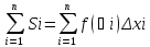 – площадьn-элемент-го
прям-ка(площадь ступенчатой ф-ры.
 i
i
Чтобы
равенство было точное, диаметр разбиения
необходимо устремить к нулю.
 .
.
Интеграл
Римана численно равен площади
криволинейной трапеции, ограниченной
сверху кривой y=f(x),
снизу – отрезком [a,b]
действительной оси и прямыми x=a
и x=b.
________________________________________________________________________
64. Свойства интеграла Римана, выражаемые равенствами.
1)
если
f(x)ϵR[a,b] и
g(x)ϵR[a,b], то
(f(x)±g(x))ϵR[a,b]
 =
=
 ±
±
Док-во:
рассмотрим интеграл
 =
= = =
= = =
= ±
± = =
= = .
.
2)
если
f(x)ϵR[a,b] и
CϵR, C=const, то
ф-я
(Cf(x))ϵR[a,b]
 =
=
 .
.
Док-во:
рассмотрим
 = [ по определению ] =
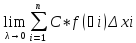 = =
= = =
= .
.
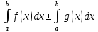
3)
если f(x)ϵR[a,b]
и a<c<b
(т.е. c-внутренняя
точка [a,b]),
то f(x)ϵR[a,c]
и f(x)ϵR[c,b]
и имеет место формула
 =
= +
+ .
.
Док-во:
разобьем отрезок [a,b]
следующим образом:
a=x0<x1<x2<…<xk=c<xk+1<…<xn=b.
 =
=
 =
= + +
+ + =
= +
+ .
.
4)
если f(x)ϵR[a,b],
то f(x)ϵR[b,a]
и имеет место формула
 =
= .
.
Док-во:
разобьем отрезки [a,b]
и [b,a]
одними и теми же точками
a=x0<x1<x2<…<xi-1<xi<…<xn=b.
тогда для [a,b]
Δxi
= xi
– xi-1
и
 ,
,
где Ѯiϵ[xi-1,
xi],
(i=2,3,…,n);
для [b,a]
Δxi=xi-1-xi=
–Δxi
, Ѯi
выберем таким же, как и в In.
In’= ’
’
= = –In
= –In
=> In
= –In’
|
 =
=
 = -(
= -( =
= .
.
5)
если f(x)ϵR[a,b],
то
 =
= =
= ,
,
т.е. интеграл не зависит от выбора
переменной интегрирования.
Док-во
следует из геометрического смысла
интеграла Римана, т.е. каждый из интегралов
определяет площадь одной и той же
криволинейной трапеции.
6)
 =b
=b
– a
(интеграл равен длине отрезка
интегрирования).
Док-во:
пусть f(x)=1.
In= =Δx1+Δx2+…+Δxn
= (x1-x0)+(x2-x1)+(x3-x2)+…+(xn-xn-1)
= xn–x0=b-a.
 =
=
 =
= = b–a.
________________________________________________________________________
Соседние файлы в предмете [НЕСОРТИРОВАННОЕ]
- #
- #
- #
- #
- #
- #
- #
- #
- #
- #
- #
