Заметки о вращении вектора кватернионом
Время на прочтение
5 мин
Количество просмотров 99K
Структура публикации
- Получение кватерниона из вектора и величины угла разворота
- Обратный кватернион
- Умножение кватернионов
- Поворот вектора
- Рысканье, тангаж, крен
- Серия поворотов
Получение кватерниона из вектора и величины угла разворота
Ещё раз – что такое кватернион? Для разработчика – это прежде всего инструмент, описывающий действие – поворот вокруг оси на заданный угол:
(w, vx, vy, vz),
где v – ось, выраженная вектором;
w – компонента, описывающая поворот (косинус половины угла).
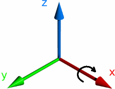
Положительное значение угла разворота означает поворот вдоль вектора по часовой стрелке, если смотреть с конца вектора в его начало.
Например, кватернион поворота вдоль оси Х на 90 градусов имеет следующие значения своих компонент: w = 0,7071; x = 0,7071; y = 0; z = 0. Левая или правая система координат, разницы нет – главное, чтобы все операции выполнялись в одинаковых системах координат, или все в левых или все в правых.
С помощью следующего кода (под рукой был Visual Basic), мы можем получить кватернион из вектора и угла разворота вокруг него:
Public Function create_quat(rotate_vector As TVector, rotate_angle As Double) As TQuat

    rotate_vector = normal(rotate_vector)
    create_quat.w = Cos(rotate_angle / 2)
    create_quat.x = rotate_vector.x * Sin(rotate_angle / 2)
    create_quat.y = rotate_vector.y * Sin(rotate_angle / 2)
    create_quat.z = rotate_vector.z * Sin(rotate_angle / 2)

End Function
В коде rotate_vector – это вектор, описывающий ось разворота, а rotate_angle – это угол разворота в радианах. Вектор должен быть нормализован. То есть его длина должа быть равна 1.
Public Function normal(v As TVector) As TVector

    Dim length As Double
    length = (v.x ^ 2 + v.y ^ 2 + v.z ^ 2) ^ 0.5
    normal.x = v.x / length
    normal.y = v.y / length
    normal.z = v.z / length

End Function
Не забывайте про ситуацию, когда длина может быть 0. Вместо ошибки вам может понадобиться обработать эту ситуацию индивидуально.
Обратный кватернион
Для поворота вектора кватернионом требуется уметь делать обратный разворот и правильно выполнять операцию умножения кватернионов. Под обратным разворотом я имею ввиду обратный кватернион, т. е. тот, который вращает в обратную сторону.
Чтобы получить обратный кватернион от заданного, достаточно развернуть вектор оси в другую сторону и при необходимости нормализовать кватернион. Нормализация кватерниона так же как и в векторах, это просто приведение к длине = 1.
Public Function quat_scale(q As TQuat, val As Double) As TQuat

    q.w = q.w * val ' x
    q.x = q.x * val ' x
    q.y = q.y * val ' y
    q.z = q.z * val ' z
    quat_scale = q

End Function

Public Function quat_length(q As TQuat) As Double

    quat_length = (q.w * q.w + q.x * q.x + q.y * q.y + q.z * q.z) ^ 0.5

End Function

Public Function quat_normalize(q As TQuat) As TQuat

    Dim n As Double
    n = quat_length(q)
    quat_normalize = quat_scale(q, 1 / n)

End Function

Public Function quat_invert(q As TQuat) As TQuat
    Dim res As TQuat

    res.w = q.w
    res.x = -q.x
    res.y = -q.y
    res.z = -q.z
    quat_invert = quat_normalize(res)
End Function
Например, если разворот вокруг оси Y на 90 градусов = (w=0,707; x = 0; y = 0,707; z=0), то обратный = (w=0,707; x = 0; y = -0,707; z=0). Казалось бы, можно инвертировать только компоненту W, но при поворотах на 180 градусов она = 0. Кватернион, который означает «нет разворота» = (w=1; x = 0; y = 0; z=0), то есть у него длина вектора оси = 0.
Умножение кватернионов
Умножение кватернионов крайне полезная штука. Результатом умножения является кватернион, который после поворота даёт такой же результат, если последовательно выполнить развороты умножаемыми кватернионами. Причём разворот будет происходить в локальной для поворачиваемого вектора системе отчёта, т. е. система отчёта поворачиваемого вектора также двигается.


Умножение кватернионов выполняется следующим образом:
Public Function quat_mul_quat(a As TQuat, b As TQuat) As TQuat

    Dim res As TQuat
    res.w = a.w * b.w - a.x * b.x - a.y * b.y - a.z * b.z
    res.x = a.w * b.x + a.x * b.w + a.y * b.z - a.z * b.y
    res.y = a.w * b.y - a.x * b.z + a.y * b.w + a.z * b.x
    res.z = a.w * b.z + a.x * b.y - a.y * b.x + a.z * b.w
    quat_mul_quat = res

End Function
Для того, чтобы умножить кватернион на 3D вектор, нужно вектор преобразовать в кватернион присвоив компоненте W = 0 и умножить кватернион на кватернион. Или подставить ноль и выразить это в виде функции:
Public Function quat_mul_vector(a As TQuat, b As TVector) As TQuat

    Dim res As TQuat
    res.w = -a.x * b.x - a.y * b.y - a.z * b.z
    res.x = a.w * b.x + a.y * b.z - a.z * b.y
    res.y = a.w * b.y - a.x * b.z + a.z * b.x
    res.z = a.w * b.z + a.x * b.y - a.y * b.x
    quat_mul_vector = res

End Function
Поворот вектора
Теперь, собственно, поворот вектора кватернионом:
Public Function quat_transform_vector(q As TQuat, v As TVector) As TVector

    Dim t As TQuat

    t = quat_mul_vector(q, v)
    t = quat_mul_quat(t, quat_invert(q))

    quat_transform_vector.x = t.x
    quat_transform_vector.y = t.y
    quat_transform_vector.z = t.z

End Function
Пример:
Вектор описывающий ось (x=1; y=0; z=1). Угол поворота 180 градусов.
Поворачиваемый вектор (x=0; y=0; z=1). Результат равен (x=1; y=0; z=0).

Рысканье, тангаж, крен
Рассмотрим инструмент формирования кватерниона с помощью поворотов вокруг одной из осей:
Рысканье = heading = yaw = вокруг оси Z; тангаж = altitude = pitch = вокруг оси Y; крен = bank = roll = вокруг оси X.
Public Function quat_from_angles_rad(angles As TKrylov) As TQuat

    Dim q_heading As TQuat
    Dim q_alt As TQuat
    Dim q_bank As TQuat
    Dim q_tmp As TQuat

    q_heading.x = 0
    q_heading.y = 0
    q_heading.z = Sin(angles.heading / 2)
    q_heading.w = Cos(angles.heading / 2)

    q_alt.x = 0
    q_alt.y = Sin(angles.altitude / 2)
    q_alt.z = 0
    q_alt.w = Cos(angles.altitude / 2)

    q_bank.x = Sin(angles.bank / 2)
    q_bank.y = 0
    q_bank.z = 0
    q_bank.w = Cos(angles.bank / 2)

    q_tmp = quat_mul_quat(q_heading, q_alt)
    quat_from_angles_rad = quat_mul_quat(q_tmp, q_bank)

End Function
И в обратную сторону, из кватерниона:
Public Function quat_to_krylov(q As TQuat) As TKrylov
    Dim qx2 As Double
    Dim qy2 As Double
    Dim qz2 As Double
    q = quat_normalize(q) 'кватернион должен быть нормализован
    qx2 = q.x * q.x
    qy2 = q.y * q.y
    qz2 = q.z * q.z
    quat_to_krylov_v3.bank = atan2(2 * (q.x * q.w + q.y * q.z), 1 - 2 * (qx2 + qy2))
    quat_to_krylov_v3.altitude = Application.WorksheetFunction.Asin(2 * (q.y * q.w - q.z * q.x))
    quat_to_krylov_v3.heading = atan2(2 * (q.z * q.w + q.x * q.y), 1 - 2 * (qy2 + qz2))
End Function
Формулы преобразования зависят от принятой системы координат.
Серия поворотов
Рассмотрим пример:
1. Первый поворот – рысканье (вокруг Z) 90 градусов по часовой;
2. Второй поворот – тангаж (вокруг Y) 90 градусов по часовой;
3. Третий поворот – крен (вокруг X) 90 градусов по часовой.
Рисунки, изображающие поворот и подписанные как «global» демонстрируют повороты относительно неподвижных осей XYZ. Такой результат мы получим, если будем использовать кватернионы разворота по отдельности. Четвёртый рисунок демонстрирует, где окажется вектор, если начальные координаты у него были X=1; Y=0; Z=0.
Рисунки, подписанные как «local» демонстрируют вращение осей вместе с самолетом. То есть все вращения происходят относительно пилота, а не относительно неподвижной системы координат. Четвёртый рисунок показывает, где окажется тот же самый вектор (1; 0; 0) в итоге всех трёх поворотов. Такой результат мы получим, перемножив кватернионы разворота и применив полученный кватернион.


Кватернионы предоставляют удобное математическое обозначение ориентации пространства и вращения объектов в этом пространстве. В сравнении с углами Эйлера кватернионы позволяют проще комбинировать вращения, а также избежать проблемы, связанной с невозможностью поворота вокруг оси независимо от совершённого вращения по другим осям (на иллюстрации). В сравнении с матрицами поворота они обладают большей вычислительной устойчивостью и могут быть более эффективными. Кватернионы нашли своё применение в компьютерной графике, робототехнике, навигации, молекулярной динамике.
Операции вращения[1][править | править код]
Представление пространства вращения[править | править код]
Кватернионы единичной нормы, согласно Гамильтону называемые также версорами (англ. versors), предоставляют алгебраический способ представления вращения в трёх измерениях. Соответствие между вращениями и кватернионами в первую очередь может быть осознано через само пространство вращения — группу SO(3).

Два вращения вокруг разных осей и на разные углы в пространстве вращений.
Любое вращение в трёхмерном пространстве — это вращение на определённый угол вокруг определённой оси. Если угол равен нулю, то выбор оси не имеет значения; таким образом, вращения на угол 0° — это точка в пространстве вращения (тождественное вращение). Для крошечного (но ненулевого) угла каждое возможное вращение на этот угол — это маленькая сфера, окружающая тождественное вращение, где каждая точка на этой сфере представляет собой ось, указывающую в определённом направлении (можно сравнить с небесной сферой). Чем больше угол вращения, тем дальше вращение от тождественного вращения; о таких вращениях можно думать как о концентрических сферах с увеличивающимся радиусом. Таким образом, вблизи тождественного вращения абстрактное пространство вращений выглядит как обычное трёхмерное пространство (которое также можно представить как центральную точку, окружённую концентрическими сферами). При увеличении угла до 360° вращения вокруг различных осей перестают расходиться и начинают становиться похожими друг на друга, становясь равными тождественному вращению, когда угол достигает 360°.

Гиперсфера вращений для вращений имеющих «горизонтальную» ось (в плоскости xy).
Мы можем увидеть похожее поведение на поверхности сферы. Если мы расположимся на северном полюсе и начнём чертить прямые линии, исходящие из него в различных направлениях (то есть линии долготы), то сначала они будут расходиться, но затем снова сойдутся на южном полюсе. Концентрические круги, получившиеся вокруг северного полюса (широты), стянутся в одну точку на южном полюсе — когда радиус сферы сравняется с расстоянием между полюсами. Если думать о разных направлениях из полюса (то есть разные долготы) как о разных осях вращения, а о разных расстояниях от полюса (то есть широтах) как о разных углах вращения, то мы получим пространство для вращений. Получившаяся сфера представляет вращение в трёхмерном пространстве, хотя является двухмерной поверхностью, что не позволяет смоделировать гиперсферу. Однако двухмерную поверхность сферы можно представлять как часть гиперсферы (как окружность является частью сферы). Мы можем взять часть, например, для представления вращения вокруг осей в плоскости xy. Важно отметить, что угол вращения до экватора равен 180° (а не 90°); до южного полюса (с северного) 360° (а не 180°).
Северный и южный полюс представляют одинаковые вращения. Это справедливо для двух любых диаметрально противоположных точек: если одна точка — это вращение на угол 


Определение пространства вращения[править | править код]
Координаты точки на поверхности сферы можно задать двумя числами, например широтой и долготой. Однако такая координата, как долгота, на северном и южном полюсах начинает вести себя неопределённо (проявляет вырожденность), хотя северный и южный полюса принципиально не отличаются от любой другой точки поверхности сферы. Это показывает, что ни одна координатная система не может двумя координатами охарактеризовать положение в пространстве. Этого можно избежать, поместив сферу в трёхмерное пространство, охарактеризовав её декартовыми координатами (w, x, y), помещая северный полюс на (w, x, y) = (1, 0, 0), южный полюс на (w, x, y) = (−1, 0, 0), а экватор на w = 0, x² + y² = 1. Точки на сфере удовлетворяют отношению w² + x² + y² = 1. В итоге получаются две степени свободы, хотя имеется три координаты. Точка (w, x, y) представляет вращение вокруг оси (x, y, 0) на угол 
Таким же образом пространство трёхмерных вращений может быть охарактеризовано тремя углами (углами Эйлера), однако любое такое представление начинает вырождаться на некоторых точках гиперсферы. Этой проблемы можно избежать, используя евклидовы координаты w, x, y, z, где w² + x² + y² + z² = 1. Точка (w, x, y, z) представляет вращение вокруг осей (x, y, z) на угол 
Коротко о кватернионах[править | править код]
Комплексное число может быть определено введением абстрактного символа i, который удовлетворяет обычным правилам алгебры, а также правилу 
.
Таким же образом кватернионы могут быть определены введением абстрактных символов i, j, k, умножение которых задаются по правилу


а умножение на вещественные числа определяются обычным образом, причём умножение полагается ассоциативным, но не коммутативным (примером некоммутативного умножения является также умножение матриц). Из этого следуют все правила кватернионной арифметики, например
.
Мнимая часть 


.
Векторное произведение некоммутативно, а произведения скаляр—скаляр и скаляр—вектор коммутативны. Из этих правил следует:
.
Обратным (слева и справа) для ненулевого кватерниона 
,
что может быть проверено прямым вычислением.
Определение пространства вращения через кватернионы[править | править код]
Допустим (w, x, y, z) — координаты вращения, согласно прежнему описанию. Тогда кватернион q можно определить как
,
где 

вращает вектор 
Можно взять композицию вращений на кватернионы, перемножив их (от порядка умножения зависит порядок вращения). Таким образом, вращения на кватернионы 


что то же самое, что и вращение на
Обращение кватерниона — это то же, что и вращение в противоположном направлении, таким образом 


Вращение на единичный кватернион[править | править код]
Пусть u — это единичный вектор (ось вращения), а 

вращает вектор v на угол α вокруг оси u. Раскрыв скобки, получаем:

где 

Получившийся результат является формулой вращения на угол α вокруг оси u.
Умножение вектора на −1, то есть взятие противоположного кватерниона, не изменяет вращение. В частности, кватернионы 1 и −1 оба определяют тождественное вращение. Более абстрактно, векторы принадлежат группе Ли SU(2), диффеоморфной 3-сфере. Эта группа двукратно накрывает пространство вращений SO(3).
Вращение четырёхмерного евклидова пространства[править | править код]
Четырёхмерное вращение описывается двумя кватернионами единичной нормы, с точностью до умножения обоих одновременно на −1.
Вариации и обобщения[править | править код]
Похожие формулы позволяют применить бикватернионы для описания преобразований Лоренца — «вращений» 4-мерного пространства Минковского.
См. также[править | править код]
- Карданов подвес
Примечания[править | править код]
- ↑
Rotations, Quaternions, and Double Groups / Altmann, Simon L. — Mineola: Dover Publications, 1986. — 317 p.
Литература[править | править код]
- В. И. Арнольд. Геометрия комплексных чисел, кватернионов и спинов. — М.: МЦНМО, 2002. — 40 с. — ISBN 5-94057-025-9.
- И. Л. Кантор, А. С. Солодовников Гиперкомплексные числа (недоступная ссылка). — М.: Наука, 1973. — 144 с.
Ссылки[править | править код]
- Shoemake, Ken. Quaternion tutorial
- Hart, Francis, Kauffman. Quaternion demo Архивная копия от 25 февраля 2009 на Wayback Machine
- Byung-Uk Lee, Unit Quaternion Representation of Rotation Архивная копия от 27 сентября 2007 на Wayback Machine
- Ibanez, Luis, Quaternion Tutorial I
- Ibanez, Luis, Quaternion Tutorial II
- Поворот в пространстве и кватернионы Архивная копия от 30 декабря 2013 на Wayback Machine
- Вращение в 3D при помощи гиперкомплексных чисел Архивная копия от 19 апреля 2014 на Wayback Machine
- Верзор // Большая советская энциклопедия : в 66 т. (65 т. и 1 доп.) / гл. ред. О. Ю. Шмидт. — М. : Советская энциклопедия, 1926—1947.
Unit quaternions, known as versors, provide a convenient mathematical notation for representing spatial orientations and rotations of elements in three dimensional space. Specifically, they encode information about an axis-angle rotation about an arbitrary axis. Rotation and orientation quaternions have applications in computer graphics,[1] computer vision, robotics,[2] navigation, molecular dynamics, flight dynamics,[3] orbital mechanics of satellites,[4] and crystallographic texture analysis.[5]
When used to represent rotation, unit quaternions are also called rotation quaternions as they represent the 3D rotation group. When used to represent an orientation (rotation relative to a reference coordinate system), they are called orientation quaternions or attitude quaternions. A spatial rotation around a fixed point of 


Compared to rotation matrices, quaternions are more compact, efficient, and numerically stable. Compared to Euler angles, they are simpler to compose. However, they are not as intuitive and easy to understand and, due to the periodic nature of sine and cosine, rotation angles differing precisely by the natural period will be encoded into identical quaternions and recovered angles in radians will be limited to ![[0,2pi]](https://wikimedia.org/api/rest_v1/media/math/render/svg/348d40bf3f8b7e1c00c4346440d7e2e4f0cc9b91)
Using quaternions as rotations[edit]

3D visualization of a sphere and a rotation about an Euler axis (
In 3-dimensional space, according to Euler’s rotation theorem, any rotation or sequence of rotations of a rigid body or coordinate system about a fixed point is equivalent to a single rotation by a given angle 
Quaternions give a simple way to encode this axis–angle representation in four numbers, and can be used to apply (calculate) the corresponding rotation to a position vector (x,y,z), representing a point relative to the origin in R3.
Euclidean vectors such as (2, 3, 4) or (ax, ay, az) can be rewritten as 2 i + 3 j + 4 k or ax i + ay j + az k, where i, j, k are unit vectors representing the three Cartesian axes (traditionally x, y, z), and also obey the multiplication rules of the fundamental quaternion units.
Therefore, a rotation of angle

can be represented by a quaternion. This can be done using an extension of Euler’s formula:

It can be shown[further explanation needed] that the desired rotation can be applied to an ordinary vector 
using the Hamilton product, where p′ = (px′, py′, pz′) is the new position vector of the point after the rotation. In a programmatic implementation, the conjugation is achieved by constructing a quaternion whose vector part is p and real part equals zero, and then performing the quaternion multiplication. The vector part of the resulting quaternion is the desired vector p′.
A geometric fact independent of quaternions is the existence of a two-to-one mapping from physical rotations to rotational transformation matrices. If 0 ⩽ 


Mathematically, this operation carries the set of all “pure” quaternions p (those with real part equal to zero)—which constitute a 3-dimensional space among the quaternions—into itself, by the desired rotation about the axis u, by the angle θ. (Each real quaternion is carried into itself by this operation. But for the purpose of rotations in 3-dimensional space, we ignore the real quaternions.)
The rotation is clockwise if our line of sight points in the same direction as
In this (which?) instance, q is a unit quaternion and

It follows that conjugation by the product of two quaternions is the composition of conjugations by these quaternions: If p and q are unit quaternions, then rotation (conjugation) by pq is
,
which is the same as rotating (conjugating) by q and then by p. The scalar component of the result is necessarily zero.
The quaternion inverse of a rotation is the opposite rotation, since 
Two rotation quaternions can be combined into one equivalent quaternion by the relation:

in which q′ corresponds to the rotation q1 followed by the rotation q2. Thus, an arbitrary number of rotations can be composed together and then applied as a single rotation. (Note that quaternion multiplication is not commutative.)
Example conjugation operation[edit]
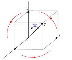
A rotation of 120° around the first diagonal permutes i, j, and k cyclically
Conjugating p by q refers to the operation p ↦ qpq−1.
Consider the rotation f around the axis 


p ↦ q p for q = 1 + i + j + k/2 on the unit 3-sphere. Note this one-sided (namely, left) multiplication yields a 60° rotation of quaternions
The length of 

If f is the rotation function,

It can be proven that the inverse of a unit quaternion is obtained simply by changing the sign of its imaginary components. As a consequence,

and

This can be simplified, using the ordinary rules for quaternion arithmetic, to

As expected, the rotation corresponds to keeping a cube held fixed at one point, and rotating it 120° about the long diagonal through the fixed point (observe how the three axes are permuted cyclically).
Quaternion-derived rotation matrix[edit]
A quaternion rotation 


Here 

This can be obtained by using vector calculus and linear algebra if we express 


this equation can be rewritten as
![{displaystyle {begin{aligned}(0, mathbf {p} ')=&((q_{r}, mathbf {v} )(0, mathbf {p} ))s(q_{r}, -mathbf {v} )\=&(q_{r}0-mathbf {v} cdot mathbf {p} , q_{r}mathbf {p} +0mathbf {v} +mathbf {v} times mathbf {p} )s(q_{r}, -mathbf {v} )\=&s(-mathbf {v} cdot mathbf {p} , q_{r}mathbf {p} +mathbf {v} times mathbf {p} )(q_{r}, -mathbf {v} )\=&s(-mathbf {v} cdot mathbf {p} q_{r}-(q_{r}mathbf {p} +mathbf {v} times mathbf {p} )cdot (-mathbf {v} ), (-mathbf {v} cdot mathbf {p} )(-mathbf {v} )+q_{r}(q_{r}mathbf {p} +mathbf {v} times mathbf {p} )+(q_{r}mathbf {p} +mathbf {v} times mathbf {p} )times (-mathbf {v} ))\=&sleft(-mathbf {v} cdot mathbf {p} q_{r}+q_{r}mathbf {v} cdot mathbf {p} , mathbf {v} left(mathbf {v} cdot mathbf {p} right)+q_{r}^{2}mathbf {p} +q_{r}mathbf {v} times mathbf {p} +mathbf {v} times left(q_{r}mathbf {p} +mathbf {v} times mathbf {p} right)right)\=&left(0, sleft(mathbf {v} otimes mathbf {v} +q_{r}^{2}mathbf {I} +2q_{r}[mathbf {v} ]_{times }+[mathbf {v} ]_{times }^{2}right)mathbf {p} right),end{aligned}}}](https://wikimedia.org/api/rest_v1/media/math/render/svg/791f3ce917350217ce39c6d61647940686c183f3)
where 

![{displaystyle [mathbf {v} ]_{times }}](https://wikimedia.org/api/rest_v1/media/math/render/svg/eb8c75c76fcc67f0d13e3298d0b6de20a0c1254e)

Since 
![{displaystyle sleft(mathbf {v} otimes mathbf {v} +q_{r}^{2}mathbf {I} +2q_{r}[mathbf {v} ]_{times }+[mathbf {v} ]_{times }^{2}right)}](https://wikimedia.org/api/rest_v1/media/math/render/svg/af9cc39b5fe69b350b9203c4f82dabeb799e0e3d)
Recovering the axis-angle representation[edit]
The expression 

![{displaystyle {begin{aligned}(a_{x},a_{y},a_{z})={}&{frac {(q_{i},q_{j},q_{k})}{sqrt {q_{i}^{2}+q_{j}^{2}+q_{k}^{2}}}}\[2pt]theta =2operatorname {atan2} &left({sqrt {q_{i}^{2}+q_{j}^{2}+q_{k}^{2}}},,q_{r}right),end{aligned}}}](https://wikimedia.org/api/rest_v1/media/math/render/svg/bc1d62fe7285e7371d40e848e6bdfca990367d8d)
where 
Care should be taken when the quaternion approaches a scalar, since due to degeneracy the axis of an identity rotation is not well-defined.
The composition of spatial rotations[edit]
A benefit of the quaternion formulation of the composition of two rotations RB and RA is that it yields directly the rotation axis and angle of the composite rotation RC = RBRA.
Let the quaternion associated with a spatial rotation R be constructed from its rotation axis S with the rotation angle 

Then the composition of the rotation RB with RA is the rotation RC = RBRA with rotation axis and angle defined by the product of the quaternions

that is

Expand this product to obtain

Divide both sides of this equation by the identity, which is the law of cosines on a sphere,

and compute

This is Rodrigues’ formula for the axis of a composite rotation defined in terms of the axes of the two rotations. He derived this formula in 1840 (see page 408).[7]
The three rotation axes A, B, and C form a spherical triangle and the dihedral angles between the planes formed by the sides of this triangle are defined by the rotation angles. Hamilton[8] presented the component form of these equations showing that the quaternion product computes the third vertex of a spherical triangle from two given vertices and their associated arc-lengths, which is also defines an algebra for points in Elliptic geometry.
Axis–angle composition[edit]
The normalized rotation axis, removing the 


Or with angle addition trigonometric substitutions…

finally normalizing the rotation axis: 

Differentiation with respect to the rotation quaternion[edit]
The rotated quaternion p’ = q p q−1 needs to be differentiated with respect to the rotating quaternion q, when the rotation is estimated from numerical optimization. The estimation of rotation angle is an essential procedure in 3D object registration or camera calibration. For unitary q and pure imaginary p, that is for a rotation in 3D space, the derivatives of the rotated quaternion can be represented using matrix calculus notation as
![{displaystyle {begin{aligned}{frac {partial mathbf {p'} }{partial mathbf {q} }}equiv left[{frac {partial mathbf {p'} }{partial q_{0}}},{frac {partial mathbf {p'} }{partial q_{x}}},{frac {partial mathbf {p'} }{partial q_{y}}},{frac {partial mathbf {p'} }{partial q_{z}}}right]=left[mathbf {pq} -(mathbf {pq} )^{*},(mathbf {pqi} )^{*}-mathbf {pqi} ,(mathbf {pqj} )^{*}-mathbf {pqj} ,(mathbf {pqk} )^{*}-mathbf {pqk} right].end{aligned}}}](https://wikimedia.org/api/rest_v1/media/math/render/svg/559fc109c72845625b201ccfa99036aa226cc204)
A derivation can be found in.[9]
Background[edit]
Quaternions[edit]
The complex numbers can be defined by introducing an abstract symbol i which satisfies the usual rules of algebra and additionally the rule i2 = −1. This is sufficient to reproduce all of the rules of complex number arithmetic: for example:

In the same way the quaternions can be defined by introducing abstract symbols i, j, k which satisfy the rules i2 = j2 = k2 = i j k = −1 and the usual algebraic rules except the commutative law of multiplication (a familiar example of such a noncommutative multiplication is matrix multiplication). From this all of the rules of quaternion arithmetic follow, such as the rules on multiplication of quaternion basis elements. Using these rules, one can show that:

The imaginary part 

Some might find it strange to add a number to a vector, as they are objects of very different natures, or to multiply two vectors together, as this operation is usually undefined. However, if one remembers that it is a mere notation for the real and imaginary parts of a quaternion, it becomes more legitimate. In other words, the correct reasoning is the addition of two quaternions, one with zero vector/imaginary part, and another one with zero scalar/real part:

We can express quaternion multiplication in the modern language of vector cross and dot products (which were actually inspired by the quaternions in the first place[10]). When multiplying the vector/imaginary parts, in place of the rules i2 = j2 = k2 = ijk = −1 we have the quaternion multiplication rule:

where:
is the resulting quaternion,
is vector cross product (a vector),
is vector scalar product (a scalar).
Quaternion multiplication is noncommutative (because of the cross product, which anti-commutes), while scalar–scalar and scalar–vector multiplications commute. From these rules it follows immediately that (see details):

The (left and right) multiplicative inverse or reciprocal of a nonzero quaternion is given by the conjugate-to-norm ratio (see details):

as can be verified by direct calculation (note the similarity to the multiplicative inverse of complex numbers).
Rotation identity[edit]
Let 

yields the vector 
![{displaystyle {begin{aligned}{vec {v}}'&={vec {v}}cos ^{2}{frac {alpha }{2}}+left({vec {u}}{vec {v}}-{vec {v}}{vec {u}}right)sin {frac {alpha }{2}}cos {frac {alpha }{2}}-{vec {u}}{vec {v}}{vec {u}}sin ^{2}{frac {alpha }{2}}\[6pt]&={vec {v}}cos ^{2}{frac {alpha }{2}}+2left({vec {u}}times {vec {v}}right)sin {frac {alpha }{2}}cos {frac {alpha }{2}}-left(left({vec {u}}times {vec {v}}right)-left({vec {u}}cdot {vec {v}}right)right){vec {u}}sin ^{2}{frac {alpha }{2}}\[6pt]&={vec {v}}cos ^{2}{frac {alpha }{2}}+2left({vec {u}}times {vec {v}}right)sin {frac {alpha }{2}}cos {frac {alpha }{2}}-left(left({vec {u}}times {vec {v}}right){vec {u}}-left({vec {u}}cdot {vec {v}}right){vec {u}}right)sin ^{2}{frac {alpha }{2}}\[6pt]&={vec {v}}cos ^{2}{frac {alpha }{2}}+2left({vec {u}}times {vec {v}}right)sin {frac {alpha }{2}}cos {frac {alpha }{2}}-left(left(left({vec {u}}times {vec {v}}right)times {vec {u}}-left({vec {u}}times {vec {v}}right)cdot {vec {u}}right)-left({vec {u}}cdot {vec {v}}right){vec {u}}right)sin ^{2}{frac {alpha }{2}}\[6pt]&={vec {v}}cos ^{2}{frac {alpha }{2}}+2left({vec {u}}times {vec {v}}right)sin {frac {alpha }{2}}cos {frac {alpha }{2}}-left(left({vec {v}}-left({vec {u}}cdot {vec {v}}right){vec {u}}right)-0-left({vec {u}}cdot {vec {v}}right){vec {u}}right)sin ^{2}{frac {alpha }{2}}\[6pt]&={vec {v}}cos ^{2}{frac {alpha }{2}}+2left({vec {u}}times {vec {v}}right)sin {frac {alpha }{2}}cos {frac {alpha }{2}}-left({vec {v}}-2{vec {u}}left({vec {u}}cdot {vec {v}}right)right)sin ^{2}{frac {alpha }{2}}\[6pt]&={vec {v}}cos ^{2}{frac {alpha }{2}}+2left({vec {u}}times {vec {v}}right)sin {frac {alpha }{2}}cos {frac {alpha }{2}}-{vec {v}}sin ^{2}{frac {alpha }{2}}+2{vec {u}}left({vec {u}}cdot {vec {v}}right)sin ^{2}{frac {alpha }{2}}\[6pt]&={vec {v}}left(cos ^{2}{frac {alpha }{2}}-sin ^{2}{frac {alpha }{2}}right)+left({vec {u}}times {vec {v}}right)left(2sin {frac {alpha }{2}}cos {frac {alpha }{2}}right)+{vec {u}}left({vec {u}}cdot {vec {v}}right)left(2sin ^{2}{frac {alpha }{2}}right)\[6pt]end{aligned}}}](https://wikimedia.org/api/rest_v1/media/math/render/svg/211d8613a1a8f990e93433cd4bd10937a2197eca)
Using trigonometric identities:
![{displaystyle {begin{aligned}{vec {v}}'&={vec {v}}left(cos ^{2}{frac {alpha }{2}}-sin ^{2}{frac {alpha }{2}}right)+left({vec {u}}times {vec {v}}right)left(2sin {frac {alpha }{2}}cos {frac {alpha }{2}}right)+{vec {u}}left({vec {u}}cdot {vec {v}}right)left(2sin ^{2}{frac {alpha }{2}}right)\[6pt]&={vec {v}}cos alpha +left({vec {u}}times {vec {v}}right)sin alpha +{vec {u}}left({vec {u}}cdot {vec {v}}right)left(1-cos alpha right)\[6pt]&={vec {v}}cos alpha +left({vec {u}}times {vec {v}}right)sin alpha +{vec {u}}left({vec {u}}cdot {vec {v}}right)-{vec {u}}left({vec {u}}cdot {vec {v}}right)cos alpha \[6pt]&=left({vec {v}}-{vec {u}}left({vec {u}}cdot {vec {v}}right)right)cos alpha +left({vec {u}}times {vec {v}}right)sin alpha +{vec {u}}left({vec {u}}cdot {vec {v}}right)\[6pt]&={vec {v}}_{bot }cos alpha +left({vec {u}}times {vec {v}}right)sin alpha +{vec {v}}_{|}end{aligned}}}](https://wikimedia.org/api/rest_v1/media/math/render/svg/48bf26328d7a60ea06272e628ae4514076e0659a)
where 

Quaternion rotation operations[edit]
A very formal explanation of the properties used in this section is given by Altman.[11]
The hypersphere of rotations[edit]
Visualizing the space of rotations[edit]
Unit quaternions represent the group of Euclidean rotations in three dimensions in a very straightforward way. The correspondence between rotations and quaternions can be understood by first visualizing the space of rotations itself.
Two separate rotations, differing by both angle and axis, in the space of rotations. Here, the length of each axis vector is relative to the respective magnitude of the rotation about that axis.
In order to visualize the space of rotations, it helps to consider a simpler case. Any rotation in three dimensions can be described by a rotation by some angle about some axis; for our purposes, we will use an axis vector to establish handedness for our angle. Consider the special case in which the axis of rotation lies in the xy plane. We can then specify the axis of one of these rotations by a point on a circle through which the vector crosses, and we can select the radius of the circle to denote the angle of rotation.
Similarly, a rotation whose axis of rotation lies in the xy plane can be described as a point on a sphere of fixed radius in three dimensions. Beginning at the north pole of a sphere in three-dimensional space, we specify the point at the north pole to be the identity rotation (a zero angle rotation). Just as in the case of the identity rotation, no axis of rotation is defined, and the angle of rotation (zero) is irrelevant. A rotation having a very small rotation angle can be specified by a slice through the sphere parallel to the xy plane and very near the north pole. The circle defined by this slice will be very small, corresponding to the small angle of the rotation. As the rotation angles become larger, the slice moves in the negative z direction, and the circles become larger until the equator of the sphere is reached, which will correspond to a rotation angle of 180 degrees. Continuing southward, the radii of the circles now become smaller (corresponding to the absolute value of the angle of the rotation considered as a negative number). Finally, as the south pole is reached, the circles shrink once more to the identity rotation, which is also specified as the point at the south pole.
Notice that a number of characteristics of such rotations and their representations can be seen by this visualization. The space of rotations is continuous, each rotation has a neighborhood of rotations which are nearly the same, and this neighborhood becomes flat as the neighborhood shrinks. Also, each rotation is actually represented by two antipodal points on the sphere, which are at opposite ends of a line through the center of the sphere. This reflects the fact that each rotation can be represented as a rotation about some axis, or, equivalently, as a negative rotation about an axis pointing in the opposite direction (a so-called double cover). The “latitude” of a circle representing a particular rotation angle will be half of the angle represented by that rotation, since as the point is moved from the north to south pole, the latitude ranges from zero to 180 degrees, while the angle of rotation ranges from 0 to 360 degrees. (the “longitude” of a point then represents a particular axis of rotation.) Note however that this set of rotations is not closed under composition. Two successive rotations with axes in the xy plane will not necessarily give a rotation whose axis lies in the xy plane, and thus cannot be represented as a point on the sphere. This will not be the case with a general rotation in 3-space, in which rotations do form a closed set under composition.
The sphere of rotations for the rotations that have a “horizontal” axis (in the xy plane).
This visualization can be extended to a general rotation in 3-dimensional space. The identity rotation is a point, and a small angle of rotation about some axis can be represented as a point on a sphere with a small radius. As the angle of rotation grows, the sphere grows, until the angle of rotation reaches 180 degrees, at which point the sphere begins to shrink, becoming a point as the angle approaches 360 degrees (or zero degrees from the negative direction). This set of expanding and contracting spheres represents a hypersphere in four dimensional space (a 3-sphere). Just as in the simpler example above, each rotation represented as a point on the hypersphere is matched by its antipodal point on that hypersphere. The “latitude” on the hypersphere will be half of the corresponding angle of rotation, and the neighborhood of any point will become “flatter” (i.e. be represented by a 3-D Euclidean space of points) as the neighborhood shrinks. This behavior is matched by the set of unit quaternions: A general quaternion represents a point in a four dimensional space, but constraining it to have unit magnitude yields a three-dimensional space equivalent to the surface of a hypersphere. The magnitude of the unit quaternion will be unity, corresponding to a hypersphere of unit radius. The vector part of a unit quaternion represents the radius of the 2-sphere corresponding to the axis of rotation, and its magnitude is the cosine of half the angle of rotation. Each rotation is represented by two unit quaternions of opposite sign, and, as in the space of rotations in three dimensions, the quaternion product of two unit quaternions will yield a unit quaternion. Also, the space of unit quaternions is “flat” in any infinitesimal neighborhood of a given unit quaternion.
Parameterizing the space of rotations[edit]
We can parameterize the surface of a sphere with two coordinates, such as latitude and longitude. But latitude and longitude are ill-behaved (degenerate) at the north and south poles, though the poles are not intrinsically different from any other points on the sphere. At the poles (latitudes +90° and −90°), the longitude becomes meaningless.
It can be shown that no two-parameter coordinate system can avoid such degeneracy. We can avoid such problems by embedding the sphere in three-dimensional space and parameterizing it with three Cartesian coordinates (w, x, y), placing the north pole at (w, x, y) = (1, 0, 0), the south pole at (w, x, y) = (−1, 0, 0), and the equator at w = 0, x2 + y2 = 1. Points on the sphere satisfy the constraint w2 + x2 + y2 = 1, so we still have just two degrees of freedom though there are three coordinates. A point (w, x, y) on the sphere represents a rotation in the ordinary space around the horizontal axis directed by the vector (x, y, 0) by an angle 
In the same way the hyperspherical space of 3D rotations can be parameterized by three angles (Euler angles), but any such parameterization is degenerate at some points on the hypersphere, leading to the problem of gimbal lock. We can avoid this by using four Euclidean coordinates w, x, y, z, with w2 + x2 + y2 + z2 = 1. The point (w, x, y, z) represents a rotation around the axis directed by the vector (x, y, z) by an angle 
Explaining quaternions’ properties with rotations[edit]
Non-commutativity[edit]
The multiplication of quaternions is non-commutative. This fact explains how the p ↦ q p q−1 formula can work at all, having q q−1 = 1 by definition. Since the multiplication of unit quaternions corresponds to the composition of three-dimensional rotations, this property can be made intuitive by showing that three-dimensional rotations are not commutative in general.
Set two books next to each other. Rotate one of them 90 degrees clockwise around the z axis, then flip it 180 degrees around the x axis. Take the other book, flip it 180° around x axis first, and 90° clockwise around z later. The two books do not end up parallel. This shows that, in general, the composition of two different rotations around two distinct spatial axes will not commute.
Orientation[edit]
The vector cross product, used to define the axis–angle representation, does confer an orientation (“handedness”) to space: in a three-dimensional vector space, the three vectors in the equation a × b = c will always form a right-handed set (or a left-handed set, depending on how the cross product is defined), thus fixing an orientation in the vector space. Alternatively, the dependence on orientation is expressed in referring to such
Alternative conventions[edit]
It is reported[12] that the existence and continued usage of an alternative quaternion convention in the aerospace and, to a lesser extent, robotics community is incurring a significant and ongoing cost [sic]. This alternative convention is proposed by Shuster M.D. in [13] and departs from tradition by reversing the definition for multiplying quaternion basis elements such that under Shuster’s convention, 

Under Shuster’s convention, the formula for multiplying two quaternions is altered such that

The formula for rotating a vector by a quaternion is altered to be
![{displaystyle {begin{aligned}mathbf {p} '_{text{alt}}={}&(mathbf {v} otimes mathbf {v} +q_{r}^{2}mathbf {I} mathbin {color {red}mathbf {-} } 2q_{r}[mathbf {v} ]_{times }+[mathbf {v} ]_{times }^{2})mathbf {p} &{text{(Alternative convention, usage discouraged!)}}\=& (mathbf {I} mathbin {color {red}mathbf {-} } 2q_{r}[mathbf {v} ]_{times }+2[mathbf {v} ]_{times }^{2})mathbf {p} &end{aligned}}}](https://wikimedia.org/api/rest_v1/media/math/render/svg/3750c56481e794e3fa99936110fba444b5c23188)
To identify the changes under Shuster’s convention, see that the sign before the cross product is flipped from plus to minus.
Finally, the formula for converting a quaternion to a rotation matrix is altered to be
![{displaystyle {begin{aligned}mathbf {R} _{alt}&=mathbf {I} mathbin {color {red}mathbf {-} } 2q_{r}[mathbf {v} ]_{times }+2[mathbf {v} ]_{times }^{2}qquad {text{(Alternative convention, usage discouraged!)}}\&={begin{bmatrix}1-2s(q_{j}^{2}+q_{k}^{2})&2(q_{i}q_{j}+q_{k}q_{r})&2(q_{i}q_{k}-q_{j}q_{r})\2(q_{i}q_{j}-q_{k}q_{r})&1-2s(q_{i}^{2}+q_{k}^{2})&2(q_{j}q_{k}+q_{i}q_{r})\2(q_{i}q_{k}+q_{j}q_{r})&2(q_{j}q_{k}-q_{i}q_{r})&1-2s(q_{i}^{2}+q_{j}^{2})end{bmatrix}}end{aligned}}}](https://wikimedia.org/api/rest_v1/media/math/render/svg/d28f0e656b8b25de89fbb55b260e7761dd7d38cf)
which is exactly the transpose of the rotation matrix converted under the traditional convention.
Software applications by convention used[edit]
The table below groups applications by their adherence to either quaternion convention:[12]
| Hamilton multiplication convention | Shuster multiplication convention |
|---|---|
|
|
While use of either convention does not impact the capability or correctness of applications thus created, the authors of [12] argued that the Shuster convention should be abandoned because it departs from the much older quaternion multiplication convention by Hamilton and may never be adopted by the mathematical or theoretical physics areas.
Comparison with other representations of rotations[edit]
Advantages of quaternions[edit]
The representation of a rotation as a quaternion (4 numbers) is more compact than the representation as an orthogonal matrix (9 numbers). Furthermore, for a given axis and angle, one can easily construct the corresponding quaternion, and conversely, for a given quaternion one can easily read off the axis and the angle. Both of these are much harder with matrices or Euler angles.
In video games and other applications, one is often interested in “smooth rotations”, meaning that the scene should slowly rotate and not in a single step. This can be accomplished by choosing a curve such as the spherical linear interpolation in the quaternions, with one endpoint being the identity transformation 1 (or some other initial rotation) and the other being the intended final rotation. This is more problematic with other representations of rotations.
When composing several rotations on a computer, rounding errors necessarily accumulate. A quaternion that is slightly off still represents a rotation after being normalized: a matrix that is slightly off may not be orthogonal any more and is harder to convert back to a proper orthogonal matrix.
Quaternions also avoid a phenomenon called gimbal lock which can result when, for example in pitch/yaw/roll rotational systems, the pitch is rotated 90° up or down, so that yaw and roll then correspond to the same motion, and a degree of freedom of rotation is lost. In a gimbal-based aerospace inertial navigation system, for instance, this could have disastrous results if the aircraft is in a steep dive or ascent.
Conversion to and from the matrix representation[edit]
From a quaternion to an orthogonal matrix[edit]
The orthogonal matrix corresponding to a rotation by the unit quaternion z = a + b i + c j + d k (with | z | = 1) when post-multiplying with a column vector is given by

This rotation matrix is used on vector w as 

where 


Also, quaternion multiplication is defined as (assuming a and b are quaternions, like z above):

where the order a, b is important since the cross product of two vectors is not commutative.
A more efficient calculation in which the quaternion does not need to be unit normalized is given by[16]

where the following intermediate quantities have been defined:

From an orthogonal matrix to a quaternion[edit]
One must be careful when converting a rotation matrix to a quaternion, as several straightforward methods tend to be unstable when the trace (sum of the diagonal elements) of the rotation matrix is zero or very small. For a stable method of converting an orthogonal matrix to a quaternion, see the Rotation matrix#Quaternion.
Fitting quaternions[edit]
The above section described how to recover a quaternion q from a 3 × 3 rotation matrix Q. Suppose, however, that we have some matrix Q that is not a pure rotation—due to round-off errors, for example—and we wish to find the quaternion q that most accurately represents Q. In that case we construct a symmetric 4 × 4 matrix

and find the eigenvector (x, y, z, w) corresponding to the largest eigenvalue (that value will be 1 if and only if Q is a pure rotation). The quaternion so obtained will correspond to the rotation closest to the original matrix Q[dubious – discuss].[17]
Performance comparisons[edit]
This section discusses the performance implications of using quaternions versus other methods (axis/angle or rotation matrices) to perform rotations in 3D.
Results[edit]
| Method | Storage |
|---|---|
| Rotation matrix | 9 |
| Quaternion | 3 or 4 (see below) |
| Angle–axis | 3 or 4 (see below) |
Only three of the quaternion components are independent, as a rotation is represented by a unit quaternion. For further calculation one usually needs all four elements, so all calculations would suffer additional expense from recovering the fourth component. Likewise, angle–axis can be stored in a three-component vector by multiplying the unit direction by the angle (or a function thereof), but this comes at additional computational cost when using it for calculations.
| Method | # multiplies | # add/subtracts | total operations |
|---|---|---|---|
| Rotation matrices | 27 | 18 | 45 |
| Quaternions | 16 | 12 | 28 |
| Method | # multiplies | # add/subtracts | # sin/cos | total operations | |
|---|---|---|---|---|---|
| Rotation matrix | 9 | 6 | 0 | 15 | |
| Quaternions * | Without intermediate matrix | 15 | 15 | 0 | 30 |
| With intermediate matrix | 21 | 18 | 0 | 39 | |
| Angle–axis | Without intermediate matrix | 18 | 13 | 2 | 30 + 3 |
| With intermediate matrix | 21 | 16 | 2 | 37 + 2 |
* Quaternions can be implicitly converted to a rotation-like matrix (12 multiplications and 12 additions/subtractions), which levels the following vectors rotating cost with the rotation matrix method.
Used methods[edit]
There are three basic approaches to rotating a vector v→:
- Compute the matrix product of a 3 × 3 rotation matrix R and the original 3 × 1 column matrix representing v→. This requires 3 × (3 multiplications + 2 additions) = 9 multiplications and 6 additions, the most efficient method for rotating a vector.
- A rotation can be represented by a unit-length quaternion q = (w, r→) with scalar (real) part w and vector (imaginary) part r→. The rotation can be applied to a 3D vector v→ via the formula
. This requires only 15 multiplications and 15 additions to evaluate (or 18 multiplications and 12 additions if the factor of 2 is done via multiplication.) This formula, originally thought to be used with axis/angle notation (Rodrigues’ formula), can also be applied to quaternion notation. This yields the same result as the less efficient but more compact formula of quaternion multiplication
.
- Use the angle/axis formula to convert an angle/axis to a rotation matrix R then multiplying with a vector, or, similarly, use a formula to convert quaternion notation to a rotation matrix, then multiplying with a vector. Converting the angle/axis to R costs 12 multiplications, 2 function calls (sin, cos), and 10 additions/subtractions; from item 1, rotating using R adds an additional 9 multiplications and 6 additions for a total of 21 multiplications, 16 add/subtractions, and 2 function calls (sin, cos). Converting a quaternion to R costs 12 multiplications and 12 additions/subtractions; from item 1, rotating using R adds an additional 9 multiplications and 6 additions for a total of 21 multiplications and 18 additions/subtractions.
| Method | # multiplies | # add/subtracts | # sin/cos | total operations | |
|---|---|---|---|---|---|
| Rotation matrix | 9n | 6n | 0 | 15n | |
| Quaternions * | Without intermediate matrix | 15n | 15n | 0 | 30n |
| With intermediate matrix | 9n + 12 | 6n + 12 | 0 | 15n + 24 | |
| Angle–axis | Without intermediate matrix | 18n | 12n + 1 | 2 | 30n + 3 |
| With intermediate matrix | 9n + 12 | 6n + 10 | 2 | 15n + 24 |
Pairs of unit quaternions as rotations in 4D space[edit]
A pair of unit quaternions zl and zr can represent any rotation in 4D space. Given a four-dimensional vector v→, and assuming that it is a quaternion, we can rotate the vector v→ like this:

The pair of matrices represents a rotation of ℝ4. Note that since 
Since the generators of the four-dimensional rotations can be represented by pairs of quaternions (as follows), all four-dimensional rotations can also be represented.
![{displaystyle {begin{aligned}mathbf {z} _{rm {l}}{vec {v}}mathbf {z} _{rm {r}}&={begin{pmatrix}1&-dt_{ab}&-dt_{ac}&-dt_{ad}\dt_{ab}&1&-dt_{bc}&-dt_{bd}\dt_{ac}&dt_{bc}&1&-dt_{cd}\dt_{ad}&dt_{bd}&dt_{cd}&1end{pmatrix}}{begin{pmatrix}w\x\y\zend{pmatrix}}\[3pt]mathbf {z} _{rm {l}}&=1+{dt_{ab}+dt_{cd} over 2}i+{dt_{ac}-dt_{bd} over 2}j+{dt_{ad}+dt_{bc} over 2}k\[3pt]mathbf {z} _{rm {r}}&=1+{dt_{ab}-dt_{cd} over 2}i+{dt_{ac}+dt_{bd} over 2}j+{dt_{ad}-dt_{bc} over 2}kend{aligned}}}](https://wikimedia.org/api/rest_v1/media/math/render/svg/d357c8e70a12570ad6275ed837bedb837306d11e)
See also[edit]
- Anti-twister mechanism
- Binary polyhedral group
- Biquaternion
- Charts on SO(3)
- Clifford algebras
- Conversion between quaternions and Euler angles
- Covering space
- Dual quaternion
- Dual-complex number
- Elliptic geometry
- Rotation formalisms in three dimensions
- Rotation (mathematics)
- Spin group
- Slerp, spherical linear interpolation
- Olinde Rodrigues
- William Rowan Hamilton
References[edit]
- ^ Shoemake, Ken (1985). “Animating Rotation with Quaternion Curves” (PDF). Computer Graphics. 19 (3): 245–254. doi:10.1145/325165.325242. Presented at SIGGRAPH ’85.
- ^ J. M. McCarthy, 1990, Introduction to Theoretical Kinematics, MIT Press
- ^ Amnon Katz (1996) Computational Rigid Vehicle Dynamics, Krieger Publishing Co. ISBN 978-1575240169
- ^ J. B. Kuipers (1999) Quaternions and rotation Sequences: a Primer with Applications to Orbits, Aerospace, and Virtual Reality, Princeton University Press ISBN 978-0-691-10298-6
- ^ Karsten Kunze, Helmut Schaeben (November 2004). “The Bingham Distribution of Quaternions and Its Spherical Radon Transform in Texture Analysis”. Mathematical Geology. 36 (8): 917–943. doi:10.1023/B:MATG.0000048799.56445.59. S2CID 55009081.
- ^ “comp.graphics.algorithms FAQ”. Retrieved 2 July 2017.
- ^ Rodrigues, O. (1840), Des lois géométriques qui régissent les déplacements d’un système solide dans l’espace, et la variation des coordonnées provenant de ses déplacements con- sidérés indépendamment des causes qui peuvent les produire, Journal de Mathématiques Pures et Appliquées de Liouville 5, 380–440.
- ^ William Rowan Hamilton (1844 to 1850) On quaternions or a new system of imaginaries in algebra, Philosophical Magazine, link to David R. Wilkins collection at Trinity College, Dublin
- ^ Lee, Byung-Uk (1991), “Differentiation with Quaternions, Appendix B” (PDF), Stereo Matching of Skull Landmarks (Ph. D. thesis), Stanford University, pp. 57–58
- ^ Altmann, Simon L. (1989). “Hamilton, Rodrigues, and the Quaternion Scandal”. Mathematics Magazine. 62 (5): 306. doi:10.2307/2689481. JSTOR 2689481.
- ^ Simon L. Altman (1986) Rotations, Quaternions, and Double Groups, Dover Publications (see especially Ch. 12).
- ^ a b c Sommer, H. (2018), “Why and How to Avoid the Flipped Quaternion Multiplication”, Aerospace, 5 (3): 72, arXiv:1801.07478, Bibcode:2018Aeros…5…72S, doi:10.3390/aerospace5030072, ISSN 2226-4310
- ^ Shuster, M.D (1993), “A Survey of attitude representations”, Journal of the Astronautical Sciences, 41 (4): 439–517, Bibcode:1993JAnSc..41..439S, ISSN 0021-9142
- ^ “MATLAB Aerospace Toolbox quatrotate”.
- ^ The MATLAB Aerospace Toolbox uses the Hamilton multiplication convention, however because it applies *passive* rather than *active* rotations, the quaternions listed are in effect active rotations using the Shuster convention.[14]
- ^ Alan Watt and Mark Watt (1992) Advanced Animation and Rendering Techniques: Theory and Practice, ACM Press ISBN 978-0201544121
- ^ Bar-Itzhack, Itzhack Y. (Nov–Dec 2000), “New method for extracting the quaternion from a rotation matrix”, Journal of Guidance, Control and Dynamics, 23 (6): 1085–1087, Bibcode:2000JGCD…23.1085B, doi:10.2514/2.4654, ISSN 0731-5090
- ^ Eberly, D., Rotation Representations and performance issues
- ^ “Bitbucket”. bitbucket.org.
Further reading[edit]
- Grubin, Carl (1970). “Derivation of the quaternion scheme via the Euler axis and angle”. Journal of Spacecraft and Rockets. 7 (10): 1261–1263. Bibcode:1970JSpRo…7.1261G. doi:10.2514/3.30149.
- Battey-Pratt, E. P.; Racey, T. J. (1980). “Geometric Model for Fundamental Particles”. International Journal of Theoretical Physics. 19 (6): 437–475. Bibcode:1980IJTP…19..437B. doi:10.1007/BF00671608. S2CID 120642923.
- Arribas, M.; Elipe, A.; Palacios, M. (2006). “Quaternions and the rotations of a rigid body”. Celest. Mech. Dyn. Astron. 96 (3–4): 239–251. Bibcode:2006CeMDA..96..239A. doi:10.1007/s10569-006-9037-6. S2CID 123591599.
External links and resources[edit]
- Shoemake, Ken. “Quaternions” (PDF). Archived (PDF) from the original on 2020-05-03.
- “Simple Quaternion type and operations in over seventy-five computer languages”. on Rosetta Code
- Hart, John C. “Quaternion Demonstrator”.
- Dam, Eik B.; Koch, Martin; Lillholm, Martin (1998). “Quaternions, Interpolation and Animation” (PDF).
- Leandra, Vicci (2001). “Quaternions and Rotations in 3-Space: The Algebra and its Geometric Interpretation” (PDF).
- Howell, Thomas; Lafon, Jean-Claude (1975). “The Complexity of the Quaternion Product, TR75-245” (PDF). Cornell University.
- Horn, Berthold K.P. (2001). “Some Notes on Unit Quaternions and Rotation” (PDF).
- Lee, Byung-Uk (1991). Unit Quaternion Representation of Rotation – Appendix A, Differentiation with Quaternions – Appendix B (PDF) (Ph. D. Thesis). Stanford University.
- Vance, Rod. “Some examples of connected Lie groups”. Archived from the original on 2018-12-15.
- “Visual representation of quaternion rotation”.
Поздравим с днём рождения Виктора Чапаева  victor_chapaev, который сподвиг меня написать данный “опус”.
Оглавление “Ликбеза по кватернионам”:
[Spoiler (click to open)]
Часть 1 – история вопроса
Часть 2 – основные операции
Часть 3 – запись вращения через кватернионы
Часть 4 – кватернионы и спиноры; порядок перемножения
Часть 5 – практическая реализация поворота
Часть 5 1/2 – введение метрики, “расстояния” между поворотами
Часть 5 3/4 – исследуем “пространство поворотов”
Часть 5 7/8 – почти изотропный ёжик
Часть 6 – поворот по кратчайшему пути
Часть 6 1/4 – кратчайший поворот в общем случае
Часть 6 2/4 – поворот, совмещающий два направления
Часть 6 3/4 – кватернион из синуса и косинуса угла
Часть 7 – интегрирование угловых скоростей, углы Эйлера-Крылова
Часть 8 – интегрирование угловых скоростей, матрицы поворота
Часть 8 1/2 – ортонормирование матрицы и уравнения Пуассона
Часть 9 – интегрирование угловых скоростей с помощью кватернионов
Часть 10 – интегрирование угловых скоростей, методы 2-го порядка
Часть 10 1/2 – интегрирование с поддержанием нормы
Часть 11 – интегрирование угловых скоростей, методы высших порядков (в разработке)
Часть 12 – навигационная задача
Часть 13 – Дэвенпорт берёт след!
Часть 14 – линейный метод Мортари-Маркли
Часть 15 – среднее от двух кватернионов
Часть 15 1/2 – проверка и усреднение кватернионов
Часть 16 – разложение кватерниона на повороты
Часть 17 – лидарная задача
Задачка к части 17
Дэвенпорт VS Мортари-Маркли
Мортари-Маркли берут реванш!
Дэвенпорт VS Мортари-Маркли, раунд 3
Мы выяснили, что такое кватернионы и почему они должны состоять именно из четырёх компонентов, узнали основные действия с ними, разобрались, как с помощью кватернионов описывается вращение в пространстве.
Теперь наконец-то поговорим о практическом их использовании – некоторые соображения, как осуществлять вращение векторов с помощью кватернионов, как интегрировать угловые скорости и как найти кратчайший поворот, переводящий один вектор (направление) в другой.
Чтобы опять не зависнуть на пару месяцев, буду писать по маленьким кусочкам. Сегодня будет уникальный материал, который вы вряд ли найдёте где-то ещё: в библиотеках раскиданы ссылки на форумы и блоги, где товарищи выводили эффективные формулы, но все эти ссылки уже мертвы. Чтобы не работать с формулами, оставленными мудрыми предками (или не воспринимать их как магические заклинания, которые надо просто выучить), автор вывел их заново и убедился в их корректности.
Реализация поворота вектора с помощью кватерниона
У нас есть кватернион Λ с единичной нормой:
и некоторый вектор , который мы записываем как кватернион с нулевой скалярной (действительной) частью:
Рассмотрим, как повернуть вектор наиболее эффективным способом.
«По определению»
Как мы уже знаем, поворот вектора можно произвести по формуле (3.2):
| (6.1) |
Если не написать специализированной функции, учитывающей, что у вектора «нет скалярной части», это потребует 32 умножения и 24 сложения, тогда как обычное умножение матрицы 3х3 на вектор требует 9 умножений и 6 сложений. Далее в тексте, для удобочитаемости будем писать в виде: 32m + 24a, что означает «32 умножения и 24 сложения».
Можно слегка упростить выражения, учитывая нулевой скалярный компонент векторов и
. Сначала вычислим промежуточный кватернион:
Выпишем выражения для компонентов кватерниона в явном виде:
Убрав умножение на нулевую скалярную часть, мы снижаем количество операций до 12m+8a. Далее, вычислим итоговый вектор, учитывая, что его скалярная часть заведомо равна нулю:
Выпишем выражения для компонентов вектора в явном виде:
Здесь мы обошлись 12m+9a. Итого, на поворот вектора требуется 24 умножения и 17 сложений – чуть лучше, чем до упрощения, но всё равно значительно более затратно, чем при умножении вектора на матрицу.
Магическая формула
Следующие формулы применены в нескольких библиотеках для работы с кватернионами, но ссылки на форум, где программист приводил вывод этих формул – давным-давно «мертвы». Для начала, сами формулы:
Как видно, используется 2 векторных умножения, 2 умножения вектора на скаляр (один из них – и вовсе число 2) и два сложения векторов. Векторное умножение требует 6m+3a, умножение на скаляр – 3m, сложение векторов – 3a.
В общей сложности, поворот вектора по (6.6) требует 18 умножений и 12 сложений, что хуже обычного матричного умножения ровно вдвое, во всяком случае, по числу операций. С другой стороны, 4 компоненты кватерниона замечательно умещаются в один регистр xmm, и при хорошей реализации на SSE полное время выполнения (включая передачу аргументов функции и возврат результата) может оказаться даже ниже.
Попробуем вывести (6.6) геометрически. Такое доказательство будет наиболее наглядным.

Мы хотим повернуть вектор вокруг оси
на угол φ. Угол φ «закодирован» внутри кватерниона:
Мы можем разложить вектор на компоненту, параллельную и перпендикулярную
(см. рисунок):
При повороте, параллельная компонента останется на том же месте, тогда как перпендикулярная повернётся, но останется в плоскости p, перпендикулярной . После поворота, этот вектор можно будет выразить следующим образом:
Вектор перпендикулярен как
, так и
, поэтому он должен быть сонаправлен их векторному произведению:
(мы можем вписать в векторное произведение полный вектор , поскольку параллельная компонента даст ноль)
Его длина составит
Мы хотим, чтобы , т.е вектор описывал бы круговое движение, сохраняющее его длину. Отсюда найдём:
Также нам необходимо выразить через исходные данные. Наиболее простой способ – через ещё одно векторное произведение:
Снова найдём длину:
Отсюда,
Наконец, выразим итоговый вектор:
Вводим вектор :
и получаем формулу (6.6).
Алгебраическое доказательство.
Ту же формулу можно вывести непосредственно из (6.1). Сначала выразим промежуточный кватернион:
Далее, найдём итоговый кватернион, который должен оказаться вектором:
Мы «выкинули» (говоря русским языком: похерили), поскольку векторное произведение ортогонально каждому из своих множителей, т.е имеет нулевое скалярное произведение с ними. Можно также сказать, что это слагаемое – не что иное, как смешанное произведение трёх векторов и равно нулю, если они линейно зависимы.
После упрощения имеем:
| (6.7) |
Заметим, что скалярная часть равна нулю, то есть перед нами действительно вектор.
Запишем формулу для двойного векторного произведения «бац минус цаб»:
| (6.8) |
но не будем убирать из (6.7) двойное векторное произведение, вместо этого выразим:
Подставляем его в (6.7):
что снова совпадает с формулой (6.6).
Вариации на тему
Может показаться, что два векторных произведения – слишком много для поворота вектора, надо обойтись одним. Да, это возможно. Подставим (6.8) в (6.7):
Первый множитель можно упростить, учитывая, что кватернион имеет единичную норму, а также вынести двойку:
| (6.9) |
Посчитаем количество операций в формуле (6.9).
Вычисление первого множителя требует 3m+1a. Затем 3m, чтобы помножить вектор на скаляр. Далее, 6m+3a для векторного произведения, 3m – умножение вектора на скаляр, 3m+2a – скалярное произведение, 3m – умножение вектора на скаляр, 3a – сложение векторов, 3a – их удвоение (либо 3m, не так уж важно в современных компьютерах), 3a – сложение векторов.
Итого: 21 умножение и 15 сложений – несколько хуже, чем по формуле (6.6).
Но как мы знаем, кроме количества арифметических операций, в современных процессорах очень важно, насколько эти операции «независимы» – требует ли каждая следующая результатов предыдущей, или можно начать выполнять их параллельно. В этом плане формула (6.9) и даже самые простые выкладки (6.3), (6.5) могут оказаться предпочтительнее.
Вычисление матрицы поворота
В компьютерной графике (и не только) часто встречается ситуация, когда необходимо повернуть множество векторов с помощью одного и того же кватерниона. В таком случае имеет смысл преобразовать кватернион в матрицу и производить поворот уже с её помощью.
Вывести матрицу поворота, соответствующую кватерниону Λ – несложно. Заметим, что все выведенные нами формулы линейны относительно входного вектора . Поэтому достаточно повернуть базисные векторы, после чего выразить поворот произвольного вектора как их взвешенную сумму.
Найдём, как повернётся вектор (1;0;0)T, он же i в кватернионной записи. Как ни странно, наиболее просто это делается «по определению». Здесь, когда используется всего один кватернион, для упрощения работы уберём индексы, записав его так:
Тогда:
Первый множитель можно упростить, учитывая единичную норму:
Повторим то же самое для вектора (0;1;0)T, он же j:
И, наконец, для вектора (0;0;1)T, он же k:
Наконец, из векторов можно составить матрицу:
На её подсчет требуется не более 13 умножений и 12 сложений. Такое количество операций достигается, если мы первоначально умножим наш кватернион на (потребует 4 умножения), благодаря чему все двойки из выражения уйдут. Дальше мы вычислим произведения x2, y2, z2, ax, ay, az, xy, xz, yz (ещё 9 умножений), и останется лишь сложить всё вместе.
Возможно, есть и более быстрые методы, но, как правило, вычисление матрицы занимает ничтожно мало времени по сравнению с последующим поворотом сотен векторов, поэтому вовсе не обязательно оптимизировать эту операцию.
Пока что кватернионы проигрывают в простоте и эффективности матрицам поворота (хотя и не значительно). Их полюбили в космической технике явно за другое… Продолжение следует.
Кватернионы. Решение одной навигационной задачи +23
Из песочницы, Алгоритмы, Matlab, Глобальные системы позиционирования
Рекомендация: подборка платных и бесплатных курсов таргетированной рекламе – https://katalog-kursov.ru/
История
Некоторое время назад я занимался одной интересной задачей, относящейся к спутниковой навигации. Используя фазовый фронт сигнала, объект навигации (ОНВ) измеряет координаты навигационных спутников (НС) в своей системе координат (локальная система, ЛСК). Также ОНВ получает значения положений НС в глобальной системе координат (ГСК), и измеряет время получения сигнала НС (рис. 1). Требовалось вычислить координаты ОНВ в ГСК и системное время, то есть решить навигационную задачу.

Задача была интересна тем, что её решение теоретически позволяет уменьшить число НС в сравнении с тем, сколько НС требуется в методах, реализованных в спутниковых системах навигации. Своё внимание в то время я в основном уделял исследованию качества измерений фазового фронта и получению навигационных уравнений для координат и времени, полагая при этом, что вычисление ориентации и координат ОНВ не вызовет особых проблем. Тем более, что на плоскости задача решалась быстро и просто.
Однако, когда я построил модель в трёхмерном пространстве, неожиданно выяснилось, что вычислить значения ориентации ОНВ при неизвестных его координатах в ГСК не получается. Несколько предпринятых попыток определить ориентацию с помощью матриц направляющих косинусов и поворотов привели к такому нагромождению тригонометрических функций, что продвигаться дальше к решению у меня не получалось. Какое-то время даже казалось, что аналитического решения вообще не существует.
Но оно, конечно, существует. Мне удалось найти решение этой задачи, используя свойства кватернионов. В этом материале я хочу описать саму задачу, ход и её решение, уделяя внимание ориентации и координатам ОНВ, и пока оставляя за рамками измерения координат по фазовому фронту.
Входные данные
Итак, входные данные:
 : вектор-столбец положения
  -го НС в ГСК,
  : номер НС,
 : вектор-столбец положения
  -го НС в координатах ЛСК; векторы
  и
и  полагаем известными; ГСК, ЛСК: правые декартовы системы координат в 3-х мерном евклидовом пространстве
  с разнонаправленными базисами
  и
и  соответственно; начала координат ГСК и ЛСК не совпадают. Нижний индекс дальше будет обозначать номер вектора, верхний – номер элемента в векторе, если только не указано явно, что это степень.
Задача

Нужно найти:
 : вектор-столбец положения ОНВ в ГСК,
 : оператор перехода от ЛСК к ГСК, который я условно назвал “оператором ориентации” (рис. 2)
Решение
Теперь ход моих рассуждений и решения.
Разложение векторов  и
и  в своих базисах:
  , где
, где  – номер НС. Базисные векторы ЛСК

где  ,
,  – множество вещественных чисел,
  . Выписывая эти коэффициенты в матрицу

получаем
![]()
полагая, что  ,
,  ,
,  . Следовательно, координаты вектора
  в базисе ГСК
  . Можно сказать, что
  является матрицей некоторого линейного оператора (или “оператора ориентации”), такого, что
  , определённого в базисе ГСК. Такой матрицей может быть матрица направляющих косинусов или любая из матриц поворотов.
Свойства произвольного евклидового пространства позволяют записать уравнение для вычисления вектора положения ОНВ:
 (1)
(1)
Неудачный поиск решения
Уравнение (1) содержит две неизвестные матричные величины  и
и  , и имеет поэтому бесконечное число решений. Аналогичное соотношение для трёх различных НС в виде
![]()
где

квадратные невырожденные матрицы, также содержат две неизвестные матричные величины  и
и  . Можно переписать (1) и (2) так, чтобы избавиться от величины
  :
:
![]()
откуда

или
![]()
где  .
.
Если бы я смог как-нибудь найти  из (3) и подставить в (1), то задача была бы решена. К примеру, была сделана попытка расписать (3) по трём НС аналогично с (2), но в итоге матрицы получались вырожденные и уравнение единственного решения поэтому не имело. Попытки расписать и решить систему уравнение вроде
![]()
приводили к тому самому нагромождению синусов и косинусов, о котором я упомянул во вступлении.
Здесь я и подумал, а получится ли найти  , если (3) или (4) записать в кватернионном виде. В итоге получилось, но продолжу по порядку.
Теория о кватернионе поворота
Два теоретических момента, которые, думаю, стоит упомянуть.
Кватернионом, как мы знаем, является математический объект вида  , где
, где  ,
,  ,
,  ,
, 
 ,
,  – скалярная часть (множитель вещественной единицы),
  – векторная часть; 1, i, j, k – вещественная и три разные мнимые единицы с таблицей умножения:
![]()
Кватернион даёт удобную возможность представления трёхмерных преобразований (вращений), определяя одновременно и ось поворота, и угол вращения. Если взять некоторый кватернион  , такой, что
  , то можно записать, что
  , и значит
  , где
, где  ,
,  . Здесь индекс в скобках обозначает номер элемента, а верхний индекс без скобки – возведение в степень. Если вектор
  представить как
![]()
где  ,
,  ,
,  , то кватернион
  запишется так:
![]()
где  . Если теперь взять произвольный кватернион
  с нулевой скалярной частью и вектором
  , то результатом операции
![]()
будет вектор  с той же длиной, что и
  , но повёрнутый на угол
  против часовой стрелки вокруг оси, направляющим вектором которой является
  . Дальше будут встречаться фразы вроде “кватернион
  выполняет поворот вектора
  “, которые, конечно, подразумевают применение кватерниона
  к вектору
  и получение
  в соответствии с (5).
Последний теоретический момент. Для обозначения разных видов умножения используются такие общеизвестные значки:  или
или  : скалярное произведение,
 : кватернионное произведение,
 : векторное произведение.
На этом с теорией всё.
Описание решения с кватернионами
Вернёмся к векторам  и
и  . Три замечания об их характере, которые потребуются дальше. Примем пока k = 1 , i = 2.
Нужные замечания
Во-первых, эти векторы являются свободными векторами, которые можно перемещать в пространстве, соблюдая параллельность перемещений.
Во-вторых, они неколлинеарны. Действительно, если бы они были коллинеарными, то (3) обращалось бы в истинное высказывание только при единичной матрице  и задачу решать не нужно было.
И, в-третьих,  . В самом деле, так как
  – это ортогональная матрица, которая не меняет длину вектора
  , то из (3) следует, что длины векторов
  и
и  равны.
Tак как в (3) длины векторов не имеют значения, для упрощения записей и решения дальше заменю векторы  и
и  их нормированными эквивалентами:

и в виде кватернионов:
![]()
Кватернионная форма основных уравнений
Выражение (3) в кватернионной форме выглядит теперь так:
![]()
где  – неизвестный кватернион, эквивалент
  , а выражение (1) так:
![]()
где  ,
,  .
.

Так как векторы  и
и  свободны, неколлинеарны, то можно совместить их концы таким образом, чтобы
  и
и  образовали угол
  на плоскости, натянутой на эти векторы (пусть эта плоскость будет
  ). Начало координат поместим в точку, общую для
  и
и  (рис. 3), и будем полагать, что значение
  известно.
Уравнение (6), аналогично уравнению (3), по-прежнему имеет бесконечное множество решений: можно найти сколько угодно различных  , которые удовлетворяют (6). Геометрически это обозначает, что можно найти бесконечное число различных прямых, вокруг которых можно выполнить вращение, совмещающее
  с
с  . На рис. 3 приведён пример, в котором поворот выполняется по кратчайшему пути вокруг прямой с направляющим вектором
  , ортогональным плоскости
  . Очевидно, что
  .
.
На рис. 4, а) и б) приведён пример, в котором вокруг некоторой оси с направляющим вектором  построен круговой конус
  с направляющими прямыми
  и
и  . Ясно, что вокруг такой оси можно сделать поворот, совмещающий
  с
с  , который будет выполнен не по кратчайшему пути (не в плоскости
  ), и угол
  , измеряемый в плоскости основания конуса
  , не будет равен
  , измеряемый в плоскости
  .
.

Чтобы найти неизвестное значение  , я добавил два новых объекта
  и
и  , получаемые из векторов
  и
и  . Выражение (6), аналогично (4), расширяется до системы уравнений
![]()
Теперь можно утверждать, что кватернион  , найденный из этой системы уравнений (8), является единственным решением, и он выполняет такой поворот в пространстве, который совмещает тройку векторов базиса ЛСК с векторами ГСК. Следовательно, его можно подставить в выражение (7) и вычислить искомое
  – положение ОНВ.
Когда я записал (8), отчего-то стало ясно, что здесь безразмерная куча тригонометрии может не возникнуть, и аналитическое решение поэтому можно будет найти более-менее просто.
Геометрия задачи

Геометрически задача теперь выглядит так. Нужно найти в пространстве такую ось, вокруг которой можно выполнить поворот, совмещающий вектор  с вектором
  , и вектор
  с вектором
  . Прямые, направляющими векторами которых являются
  (или
(или  ) и
) и  (или
(или  ), образуют два различных круговых конуса
  ,
,  . Эти конусы имеют общую ось, направляющим вектором которой является искомый
  . При этом повороты
  к
к  , i = 1, 2, будут выполняться не по кратчайшему пути, и поэтому углы
  , измеренные в плоскости оснований конусов
  , будут отличаться от углов
  (рис. 5).
Здесь и далее нам понадобятся два таких утверждения.
Утверждение 1. Угол поворота вокруг биссектрисы  такого, который совмещает
  с
с  , равен
  (рис. 4, в), г)).
Утверждение 2. Поворот, который совмещает  с
с  , i = 1, 2, вокруг некоторой прямой можно сделать тогда и только тогда, когда эта прямая лежит в плоскости, натянутой на
  и
и  (плоскость
  ), рис. 6). Вокруг любой другой прямой такой поворот выполнить нельзя.

Для доказательства этих утверждений нужно рассмотреть свойства кругового конуса  , образованного линией, направляющий вектор которой равен
  (или
(или  ), а ось лежит в плоскости
  .
.
Очевидно, что ось, вокруг которой можно сделать такой поворот, который совместит  с
с  , i = 1, 2, будет одновременно принадлежать обеим плоскостям
  , то есть будет совпадать с линией их пересечения. Поэтому вектор
  будем искать из уравнения линии пересечения плоскостей
  (рис. 7).

Эта прямая не будет совпадать с прямыми, определяемые направляющими векторами  . Проходя через начало координат, она образует некоторый угол
  с вектором
  , и угол
  с вектором
  (рис. 8). Оба этих угла нам пока неизвестны и
  .
.

Посмотрим на рис. 8. Если взять некоторый кватернион  , который поворачивает вектор
  на
на  в плоскости
  , т.е.
![]()
и повернуть его вокруг начала координат на угол  в плоскости
  , то из
![]()
мы получим вектор  , который в свою очередь является кватернионом поворота на угол
  для вектора
  , причём
  при этом будет описывать дугу в пространстве. Поворот
  к
к  может быть выполнен кватернионом
  , который мы найдём чуть позже из условия его ортогональности к плоскости
  .
.
Из утверждения 2 следует, что вектор  может быть совмещён с
  вращением вокруг оси с направляющим вектором
  на некоторый угол
  , который, очевидно, функционально зависит от
  . Поэтому, зная
  и зависимость
  , мы сможем построить из кватерниона
  кватернион
  , являющийся решением задачи.
Зависимость  мы найдём немного позже из простых тригонометрических соотношений.
Угол  будем искать из следующих соображений. Так как
  ортогонален одновременно
  и
и  , то результат векторного произведения
  будет сонаправлен с
  . Обозначим
![]()
и запишем такое скалярное произведение:  . Отметим, что направление
  не зависит ни от
  , ни от
  . Поэтому для вычисления
  примем
  и
и  , то есть угол, при котором
  . Следовательно, в записанном выше скалярном произведении остаётся одна переменная
  , которую можно вычислить, решив уравнение
![]()
полагая, что  . Теперь, зная
  , зависимость
  и вектор
  , искомый кватернион
  будет выглядеть так:
![]()
Осталось найти каждый из описанных выше элементов, чтобы решить задачу. Заметим, что объекты  ,
,  ,
,  ,
,  ,
,  ,
,  определяются аналогично. Поэтому далее нижний индекс “1” или “2” буду заменять на ” i “, подразумевая, что i = 1, 2 .
Кватернионы, которые будем искать
Ещё раз перечислим кватернионы и векторы, которые мы сейчас будем строить для получения решения:
-
кватернион
 : совмещает вектор
  с
с  по кратчайшей траектории,
 -
кватернион
 : направляющий вектор биссектрисы угла между векторами
  и
и  ; векторы
  и
и  определяют плоскость
  , в которой лежит искомый кватернион
  ,
, -
кватернион
 : сонаправлен с
  ; модуль векторной части
  равен 1,
 -
кватернион
 : поворачивает вектор
  в плоскости
  на угол
  ; значение
  неизвестно,
 -
зависимость
 : вычисляет
  для построения искомого кватерниона
  из
из  ,
, -
кватернион
 : получен поворотом вектора
  в плоскости
  на угол
  ; из
; из  будет получено решение,
 -
кватернион
 : нужен для вычисления угла
  ,
, -
и, наконец, результирующий кватернион
 : получается из
  , учитывая найденные
  и
и  .
.
Кватернион 
Найдём кватернион  , который совмещает
  с
с  по кратчайшей траектории. Вектор
  перемещается в плоскости
  , а ось поворота перпендикулярна
  и проходит через точку начала координат (рис. 3). Направляющий вектор этой оси может быть равен
  . Так как
  , и
, и  , то:
, то:
![]()
где  – единичный вектор, равный

где
![]()
Произведение  может представлять собой векторную часть некоторого кватерниона
  , который выполняет поворот вектора
  на угол
  в плоскости
  :
:  . Поэтому кватернион поворота
  на угол
  равен
равен
![]()
и
![]()
Кватернион 
Найдём кватернион  . Он может быть получен из преобразования
![]()
где  – кватернион, выполняющий поворот вектора
  на угол
  . Учитывая (17), он равен
![]()
Подставим  из (19) в (18), выполним кватернионные умножения и, учитывая (14), получим:

Применяя правило “БАЦ минус ЦАБ” и упрощая, получаем
![]()
Заметим, что  .
.
Зависимость 

Найдём зависимость  . Возьмём конус
  из рис. 6, для удобства развернём его основанием вниз и изобразим все основные векторы и углы (рис. 9). Также добавим угол
  .
.
Будем находить зависимость угла  , соответствующего углу поворота вокруг
  от
от  к
к  , от значения угла
  , то есть от угла наклона
  к плоскости векторов
  ,
,  (т.е. к плоскости
  ). Заметим, что при
  поворот выполняется по кратчайшей траектории вокруг
  .
.
Из соотношений прямоугольных треугольников запишем:
![]()
откуда  . Так как
  ), то
), то
![]()
откуда
![]()
Из выражения (21) видно, что при  значение
  , а при
  значение
  , что согласуется с утверждением 1. Заметим также, что угол
  не зависит от длин векторов, а угол
  полагается известным.
Кватернион 
Продолжим. Построим кватернион  . Поскольку он выполняет поворот
  на угол
  в плоскости
  , то
, то
![]()
полагая, что  ,
,  . Учитывая (9), (18), выполнив некоторые преобразования, получим

После упрощающих тригонометрических преобразований, подставляя в (22), получаем
![]()
при этом  .
.
Кватернион 
Найдём кватернион  . Выше мы записали выражение (9), которое определяет
  . Приведём его здесь ещё раз:
  . Подставляя сюда полученный результат (23) и выражение (9), после преобразований получим:
![]()
где  ,
,  ,
,  . Упрощая, получаем:
![]()
при этом  .
.
Кватернион 
Получим кватернион  . Как мы указывали выше, вектор этого кватерниона ортогонален каждому из векторов
  и
и  , то есть
  (выражение (11)), и при этом
  . Также мы отмечали, что угол
  не меняет направление вектора
  , и поэтому можно выбрать такое
  , при котором длина
  максимальна. Учитывая (23) при
  , получаем:
![]()
следовательно,
![]()
Нормированное значение
![]()
Угол 
Подставляем результаты в выражение (12) и получаем уравнение, которое нужно решить относительно  :
:
![]()
После преобразований получаем это уравнение в форме  , которое и решаем:
![]()
где

Решение
Зная  , можно построить кватернион
  из (24), подставить его в (13) и записать результат в виде:
![]()
где
![]()
а  вычисляется из выражения (29).
Послесловие
Задача решена. Я попытался упростить итоговое выражение (30), но пока не получилось. В моделях оно работает, поэтому пока оставлю, как есть. На рис. 10 приведён простой пример нахождения ориентации ЛСК для того, чтобы затем определить  .
.

Вначале положение ЛСК  неизвестно, и мы полагаем, что оно может быть любым или, например, совпадающим с ГСК (то есть, мы “думаем”, что оно совпадает, а на самом деле это не так). Измеренные координаты НС1′, НС2′ и НС3′ существенно отличаются от истинных положений НС1, НС2 и НС3 (рис. 10, а)). Зная координаты НС в ГСК, вычисляется кватернион поворота
  по (30) и выполняется вращение. На рис. 10, б) показано дискретное вращение с интервалом 10 градусов от старого положения ЛСК к истинному. При этом измеренные координаты НС (показаны светло-серым цветом) всё более приближаются к истинным. На рис. 10, в) показано вычисленное истинное положение ЛСК, и мы теперь можем определить
  , то есть решить навигационную задачу (точнее, часть навигационной задачи, связанной с определением координат).
На этом пока всё. Отмечу только, что в ближайшем будущем я попробую поработать над одним недостатком выражения (30). При  близким к нулю, то есть когда ориентации ГСК и ЛСК мало отличаются, кватернион
  вычисляется с ошибкой из-за множителя
  . Это может приводить к значительным ошибкам вычисления ориентации ЛСК и, как результат, ошибкам определения положения
  . Об этом в следующем материале.
