Another approach (more words, less code) that may help:
The locations of local maxima and minima are also the locations of the zero crossings of the first derivative. It is generally much easier to find zero crossings than it is to directly find local maxima and minima.
Unfortunately, the first derivative tends to “amplify” noise, so when significant noise is present in the original data, the first derivative is best used only after the original data has had some degree of smoothing applied.
Since smoothing is, in the simplest sense, a low pass filter, the smoothing is often best (well, most easily) done by using a convolution kernel, and “shaping” that kernel can provide a surprising amount of feature-preserving/enhancing capability. The process of finding an optimal kernel can be automated using a variety of means, but the best may be simple brute force (plenty fast for finding small kernels). A good kernel will (as intended) massively distort the original data, but it will NOT affect the location of the peaks/valleys of interest.
Fortunately, quite often a suitable kernel can be created via a simple SWAG (“educated guess”). The width of the smoothing kernel should be a little wider than the widest expected “interesting” peak in the original data, and its shape will resemble that peak (a single-scaled wavelet). For mean-preserving kernels (what any good smoothing filter should be) the sum of the kernel elements should be precisely equal to 1.00, and the kernel should be symmetric about its center (meaning it will have an odd number of elements.
Given an optimal smoothing kernel (or a small number of kernels optimized for different data content), the degree of smoothing becomes a scaling factor for (the “gain” of) the convolution kernel.
Determining the “correct” (optimal) degree of smoothing (convolution kernel gain) can even be automated: Compare the standard deviation of the first derivative data with the standard deviation of the smoothed data. How the ratio of the two standard deviations changes with changes in the degree of smoothing cam be used to predict effective smoothing values. A few manual data runs (that are truly representative) should be all that’s needed.
All the prior solutions posted above compute the first derivative, but they don’t treat it as a statistical measure, nor do the above solutions attempt to performing feature preserving/enhancing smoothing (to help subtle peaks “leap above” the noise).
Finally, the bad news: Finding “real” peaks becomes a royal pain when the noise also has features that look like real peaks (overlapping bandwidth). The next more-complex solution is generally to use a longer convolution kernel (a “wider kernel aperture”) that takes into account the relationship between adjacent “real” peaks (such as minimum or maximum rates for peak occurrence), or to use multiple convolution passes using kernels having different widths (but only if it is faster: it is a fundamental mathematical truth that linear convolutions performed in sequence can always be convolved together into a single convolution). But it is often far easier to first find a sequence of useful kernels (of varying widths) and convolve them together than it is to directly find the final kernel in a single step.
Hopefully this provides enough info to let Google (and perhaps a good stats text) fill in the gaps. I really wish I had the time to provide a worked example, or a link to one. If anyone comes across one online, please post it here!
Gradient Descent is an iterative algorithm that is used to minimize a function by finding the optimal parameters. Gradient Descent can be applied to any dimension function i.e. 1-D, 2-D, 3-D. In this article, we will be working on finding global minima for parabolic function (2-D) and will be implementing gradient descent in python to find the optimal parameters for the linear regression equation (1-D). Before diving into the implementation part, let us make sure the set of parameters required to implement the gradient descent algorithm. To implement a gradient descent algorithm, we require a cost function that needs to be minimized, the number of iterations, a learning rate to determine the step size at each iteration while moving towards the minimum, partial derivatives for weight & bias to update the parameters at each iteration, and a prediction function.
Till now we have seen the parameters required for gradient descent. Now let us map the parameters with the gradient descent algorithm and work on an example to better understand gradient descent. Let us consider a parabolic equation y=4x2. By looking at the equation we can identify that the parabolic function is minimum at x = 0 i.e. at x=0, y=0. Therefore x=0 is the local minima of the parabolic function y=4x2. Now let us see the algorithm for gradient descent and how we can obtain the local minima by applying gradient descent:
Algorithm for Gradient Descent
Steps should be made in proportion to the negative of the function gradient (move away from the gradient) at the current point to find local minima. Gradient Ascent is the procedure for approaching a local maximum of a function by taking steps proportional to the positive of the gradient (moving towards the gradient).
repeat until convergence
{
    w = w - (learning_rate * (dJ/dw))
    b = b - (learning_rate * (dJ/db))
}
Step 1: Initializing all the necessary parameters and deriving the gradient function for the parabolic equation 4x2. The derivative of x2 is 2x, so the derivative of the parabolic equation 4x2 will be 8x.
x0 = 3 (random initialization of x)
learning_rate = 0.01 (to determine the step size while moving towards local minima)
gradient =  (Calculating the gradient function)
Step 2: Let us perform 3 iterations of gradient descent:
For each iteration keep on updating the value of x based on the gradient descent formula.
Iteration 1:
    x1 = x0 - (learning_rate * gradient)
    x1 = 3 - (0.01 * (8 * 3))
    x1 = 3 - 0.24
    x1 = 2.76

Iteration 2:
    x2 = x1 - (learning_rate * gradient)
    x2 = 2.76 - (0.01 * (8 * 2.76))
    x2 = 2.76 - 0.2208
    x2 = 2.5392

Iteration 3:
    x3 = x2 - (learning_rate * gradient)
    x3 = 2.5392 - (0.01 * (8 * 2.5392))
    x3 = 2.5392 - 0.203136
    x3 = 2.3360
From the above three iterations of gradient descent, we can notice that the value of x is decreasing iteration by iteration and will slowly converge to 0 (local minima) by running the gradient descent for more iterations. Now you might have a question, for how many iterations we should run gradient descent?
We can set a stopping threshold i.e. when the difference between the previous and the present value of x becomes less than the stopping threshold we stop the iterations. When it comes to the implementation of gradient descent for machine learning algorithms and deep learning algorithms we try to minimize the cost function in the algorithms using gradient descent. Now that we are clear with the gradient descent’s internal working, let us look into the python implementation of gradient descent where we will be minimizing the cost function of the linear regression algorithm and finding the best fit line. In our case the parameters are below mentioned:
Prediction Function
The prediction function for the linear regression algorithm is a linear equation given by y=wx+b.
prediction_function (y) = (w * x) + b
Here, x is the independent variable
      y is the dependent variable
      w is the weight associated with input variable
      b is the bias
Cost Function
The cost function is used to calculate the loss based on the predictions made. In linear regression, we use mean squared error to calculate the loss. Mean Squared Error is the sum of the squared differences between the actual and predicted values.
Cost Function (J) = 
Here, n is the number of samples
Partial Derivatives (Gradients)
Calculating the partial derivatives for weight and bias using the cost function. We get:


Parameter Updation
Updating the weight and bias by subtracting the multiplication of learning rates and their respective gradients.
w = w - (learning_rate * (dJ/dw))
b = b - (learning_rate * (dJ/db))
Python Implementation for Gradient Descent
In the implementation part, we will be writing two functions, one will be the cost functions that take the actual output and the predicted output as input and returns the loss, the second will be the actual gradient descent function which takes the independent variable, target variable as input and finds the best fit line using gradient descent algorithm. The iterations, learning_rate, and stopping threshold are the tuning parameters for the gradient descent algorithm and can be tuned by the user. In the main function, we will be initializing linearly related random data and applying the gradient descent algorithm on the data to find the best fit line. The optimal weight and bias found by using the gradient descent algorithm are later used to plot the best fit line in the main function. The iterations specify the number of times the update of parameters must be done, the stopping threshold is the minimum change of loss between two successive iterations to stop the gradient descent algorithm.
Python3
import numpy as np
import matplotlib.pyplot as plt
def mean_squared_error(y_true, y_predicted):
cost = np.sum((y_true-y_predicted)**2) / len(y_true)
return cost
def gradient_descent(x, y, iterations = 1000, learning_rate = 0.0001,
stopping_threshold = 1e-6):
current_weight = 0.1
current_bias = 0.01
iterations = iterations
learning_rate = learning_rate
n = float(len(x))
costs = []
weights = []
previous_cost = None
for i in range(iterations):
y_predicted = (current_weight * x) + current_bias
current_cost = mean_squared_error(y, y_predicted)
if previous_cost and abs(previous_cost-current_cost)<=stopping_threshold:
break
previous_cost = current_cost
costs.append(current_cost)
weights.append(current_weight)
weight_derivative = -(2/n) * sum(x * (y-y_predicted))
bias_derivative = -(2/n) * sum(y-y_predicted)
current_weight = current_weight - (learning_rate * weight_derivative)
current_bias = current_bias - (learning_rate * bias_derivative)
print(f"Iteration {i+1}: Cost {current_cost}, Weight
{current_weight}, Bias {current_bias}")
plt.figure(figsize = (8,6))
plt.plot(weights, costs)
plt.scatter(weights, costs, marker='o', color='red')
plt.title("Cost vs Weights")
plt.ylabel("Cost")
plt.xlabel("Weight")
plt.show()
return current_weight, current_bias
def main():
X = np.array([32.50234527, 53.42680403, 61.53035803, 47.47563963, 59.81320787,
55.14218841, 52.21179669, 39.29956669, 48.10504169, 52.55001444,
45.41973014, 54.35163488, 44.1640495 , 58.16847072, 56.72720806,
48.95588857, 44.68719623, 60.29732685, 45.61864377, 38.81681754])
Y = np.array([31.70700585, 68.77759598, 62.5623823 , 71.54663223, 87.23092513,
78.21151827, 79.64197305, 59.17148932, 75.3312423 , 71.30087989,
55.16567715, 82.47884676, 62.00892325, 75.39287043, 81.43619216,
60.72360244, 82.89250373, 97.37989686, 48.84715332, 56.87721319])
estimated_weight, estimated_bias = gradient_descent(X, Y, iterations=2000)
print(f"Estimated Weight: {estimated_weight}nEstimated Bias: {estimated_bias}")
Y_pred = estimated_weight*X + estimated_bias
plt.figure(figsize = (8,6))
plt.scatter(X, Y, marker='o', color='red')
plt.plot([min(X), max(X)], [min(Y_pred), max(Y_pred)], color='blue',markerfacecolor='red',
markersize=10,linestyle='dashed')
plt.xlabel("X")
plt.ylabel("Y")
plt.show()
if __name__=="__main__":
main()
Output:
Iteration 1: Cost 4352.088931274409, Weight 0.7593291142562117, Bias 0.02288558130709
Iteration 2: Cost 1114.8561474350017, Weight 1.081602958862324, Bias 0.02918014748569513
Iteration 3: Cost 341.42912086804455, Weight 1.2391274084945083, Bias 0.03225308846928192
Iteration 4: Cost 156.64495290904443, Weight 1.3161239281746984, Bias 0.03375132986012604
Iteration 5: Cost 112.49704004742098, Weight 1.3537591652024805, Bias 0.034479873154934775
Iteration 6: Cost 101.9493925395456, Weight 1.3721549833978113, Bias 0.034832195392868505
Iteration 7: Cost 99.4293893333546, Weight 1.3811467575154601, Bias 0.03500062439068245
Iteration 8: Cost 98.82731958262897, Weight 1.3855419247507244, Bias 0.03507916814736111
Iteration 9: Cost 98.68347500997261, Weight 1.3876903144657764, Bias 0.035113776874486774
Iteration 10: Cost 98.64910780902792, Weight 1.3887405007983562, Bias 0.035126910596389935
Iteration 11: Cost 98.64089651459352, Weight 1.389253895811451, Bias 0.03512954755833985
Iteration 12: Cost 98.63893428729509, Weight 1.38950491235671, Bias 0.035127053821718185
Iteration 13: Cost 98.63846506273883, Weight 1.3896276808137857, Bias 0.035122052266051224
Iteration 14: Cost 98.63835254057648, Weight 1.38968776283053, Bias 0.03511582492978764
Iteration 15: Cost 98.63832524036214, Weight 1.3897172043139192, Bias 0.03510899846107016
Iteration 16: Cost 98.63831830104695, Weight 1.389731668997059, Bias 0.035101879159522745
Iteration 17: Cost 98.63831622628217, Weight 1.389738813163012, Bias 0.03509461674147458
Estimated Weight: 1.389738813163012
Estimated Bias: 0.03509461674147458
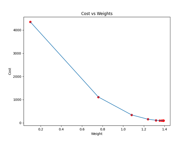
Cost function approaching local minima
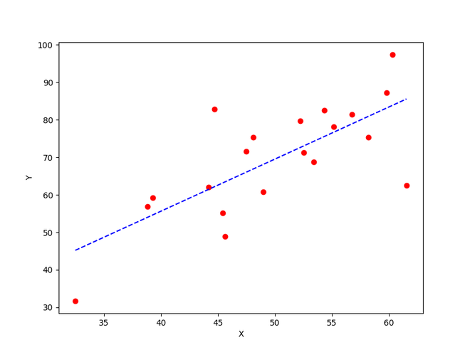
The best fit line obtained using gradient descent
Problem Formulation
The extreme location of a function is the value x at which the value of the function is the largest or smallest over a given interval or the entire interpretation range.
There is a local maximum of f(x) in x0 if there is an environment such that for any x in this environment f(x) ≥ f(x0). There is a local minimum of f(x) in x0 if there is an environment such that for any x in this environment f(x) ≤ f(x0).
For a function f(x) can have several local extrema. All global extreme values are also local, but vice versa of course this is not true.
These values are often called “peaks” because they are the tops of the “hills” and “valleys” that appear on the graph of the function.
The practical application of these points is essential, for example in image processing and signal processing, for example in detecting extraterrestrial messages! 🙂
In this article, we’ll look at some simple ways to find dips in a NumPy array with only NumPy‘s built-in functions, or using scipy library.
Find All the Dips in a 1D NumPy Array
Local minimum dips are points surrounded by larger values on both sides.
Of course, there are many ways to solve the problem, you can use pure numpy, or you can loop through the data, or you can use the SciPy library.
I found a great solution on Github, a work by Benjamin Schmidt, which shows the definition of the local extremum very well:
Method 1: Using numpy’s numpy.where
import numpy as np
import matplotlib.pyplot as plt

x = np.linspace (0, 50, 1000)
y = 0.75 * np.sin(x)

peaks = np.where((y[1:-1] > y[0:-2]) * (y[1:-1] > y[2:]))[0] + 1
dips = np.where((y[1:-1] < y[0:-2]) * (y[1:-1] < y[2:]))[0] + 1


plt.plot (x, y)
plt.plot (x[peaks], y[peaks], 'o')
plt.plot (x[dips], y[dips], 'o')

plt.show()
The above makes a list of all indices where the value of y[i] is greater than both of its neighbors. It does not check the endpoints, which only have one neighbor each.
The extra +1 at the end is necessary because where finds the indices within the slice y[1:-1], not the full array y. The index [0] is necessary because where returns a tuple of arrays, where the first element is the array we want.
We use the Matplotlib library to make a graph. For a complete guide, see the Finxter Computer Science Academy course on Matplotlib.
Method 2: Using numpy.diff
Another simple approach of the solution is using NumPy’s built-in function numpy.diff.
import numpy as np


# define an array
arr = np.array([1, 3, 7, 1, 2, 6, 0, 1, 6, 0, -2, -5, 18])


# What "numpy.diff" does, and what is the type of the result?
#print((np.diff(arr), type(np.diff(arr))))


# What "numpy.sign" does?
#print(np.sign(np.diff(arr)))


peaks = np.diff(np.sign(np.diff(arr)))
#print(peaks)


local_minima_pos = np.where(peaks == 2)[0] + 1
print(local_minima_pos)
We define a 1D array “arr” and then comes a one-liner. In it, first, we calculate the differences between each element with np.diff(arr).
After that, we use the „numpy.sign” function on that array, hence we get the sign of the differences, i.e., -1 or 1.
Then we use the function “numpy.sign” on the array to get the sign of the differences, i.e., -1 or 1.
The whole thing is passed into another function “numpy.diff” which returns +2 or -2 or 0. A value of 0 indicates a continuous decrease or increase, -2 indicates a maximum, and +2 indicates a minimum.
Now, we have the peaks and numpy.where tells us the positions. Note the +1 at the end of the line, this is because the 0th element of the peaks array is the difference between the 0th and 1st element of the arr array. The index [0] is necessary because „numpy.where” returns a tuple of arrays—the first element is the array we want.
Method 3: Solution with scipy
In the last example, I want to show how the SciPy library can be used to solve the problem in a single line.
import numpy as np
from scipy.signal import argrelextrema

x = np.linspace (0, 50, 100)
y = np.sin(x)

#print(y)

print(argrelextrema(y, np.less))
Find all the Dips in a 2D NumPy Array
2D arrays can be imagined as digital (grayscale) images built up from pixels. For each pixel, there is a value representing the brightness. These values are represented in a matrix where the pixel positions are mapped on the two axes. If we want to find the darkest points, we need to examine the neighbors of each point.
Method 1: Naive Approach
This can be done by checking for each cell by iterating over each cell [i,j]. If all the neighbours are higher than the actual cell, then it is a local minima. This approach is not optimal, since redundant calculations are performed on the neighbouring cells.
Method 2: Using the „and” Operator
The first step is to add the global maximum of the array to the surrounding of the array so that when the element-wise test reaches the “edge” of the array, the comparison works. Since the current cell is compared to the previous and next cells, an error message would be generated at the end of the axes. The local minimum will always be less than the global maximum, so our comparison will work fine. We then go through the cells of the array, performing the comparison.
To reduce redundant computations, we use a logical “and” operation, so that if one of the conditions is not met, the algorithm will not perform the further comparison.
The indices of elements matching the criteria are collected in a tuple list. Note that the indices of the original array are different from the indices of the expanded array! Therefore we reduce the indices by -1.
import numpy as np


data = np.array([[-210, 2, 0, -150],
                 [4, -1, -60, 10],
                 [0, 0, -110, 10],
                 [-50, -11, -2, 10]])


a = np.pad(data, (1, 1),
           mode='constant',
           constant_values=(np.amax(data), np.amax(data)))
loc_min = []
rows = a.shape[0]
cols = a.shape[1]


for ix in range(0, rows - 1):
    for iy in range(0, cols - 1):
        if a[ix, iy] < a[ix, iy + 1] and a[ix, iy] < a[ix, iy - 1] and
           a[ix, iy] < a[ix + 1, iy] and a[ix, iy] < a[ix + 1, iy - 1] and
           a[ix, iy] < a[ix + 1, iy + 1] and a[ix, iy] < a[ix - 1, iy] and
           a[ix, iy] < a[ix - 1, iy - 1] and a[ix, iy] < a[ix - 1, iy + 1]:
            temp_pos = (ix-1, iy-1)
            loc_min.append(temp_pos)


print(loc_min)
# [(0, 0), (0, 3), (2, 2), (3, 0)]
Method 3: Using scipy’s ndimage minimum filter
Fortunately, there is also a SciPy function for this task:
scipy.ndimage.minimum_filter(input,
                             size = None,
                             footprint = None,
                             output = None,
                             mode = 'reflect',
                             cval = 0.0,
                             origin = 0)
It creates a Boolean array, where local minima are ’True’.
- The ‘
size‘ parameter is used, which specifies the shape taken from the input array at each element position, to define the input to the filter function. - The
footprintis a Boolean array that specifies (implicitly) a shape, but also which of the elements within the shape are passed to the filter function. - The
modeparameter determines how the input array is extended when the filter overlaps a border. By passing a sequence of modes of length equal to the number of dimensions of the input array, different modes can be specified along each axis. - Here, the ‘
constant‘ parameter is specified, so the input is expanded by filling all values beyond the boundary with the same constant value specified by the ‘cval‘ parameter. The value of ‘cval‘ is set to the global maximum, ensuring that any local minimum on the boundary is also found.
See the SciPy documentation for more detailed information on how the filters work. We then check which cells are “True”, so that all the local minimum indices are in an array.
import numpy as np
from scipy.ndimage.filters import minimum_filter


data = np.array([[2, 100, 1000, -5],
		[-10, 9, 1800, 0],
		[112, 10, 111, 100],
		[50, 110, 50, 140]])


minima = (data == minimum_filter(data, 3, mode='constant', cval=0.0))
# print(data)
# print(minima)


res = np.where(1 == minima)
print(res)
Performance Evaluation
To learn about which method is faster, I’ve evaluated the runtime performance in an experimental setting. The result shows that the minimum filter method is significantly faster than the “for loop” method:

Here’s the code generating this output:
import numpy as np
import time as tm
import matplotlib.pyplot as plt
from scipy.ndimage.filters import minimum_filter

data = np.random.rand(50, 50)

a = np.pad(data, (1, 1), mode='constant',
           constant_values=(np.amax(data), np.amax(data)))
loc_min = []
rows = a.shape[0]
cols = a.shape[1]


begin1 = tm.time()

for ix in range(0, rows - 1):
    for iy in range(0, cols - 1):
                if (a[ix, iy] < a[ix, iy + 1]
                    and a[ix, iy] < a[ix, iy - 1]
                    and a[ix, iy] < a[ix + 1, iy]
                    and a[ix, iy] < a[ix + 1, iy - 1]
                    and a[ix, iy] < a[ix + 1, iy + 1]
                    and a[ix, iy] < a[ix - 1, iy]
                    and a[ix, iy] < a[ix - 1, iy - 1]
                    and a[ix, iy] < a[ix - 1, iy + 1]):
                    temp_pos = (ix-1, iy-1)
                    loc_min.append(temp_pos)


end1 = tm.time()
dt1 = (end1 - begin1)

print(f"Total runtime of the program is {end1 - begin1}")

begin2 = tm.time()

minima = (data == minimum_filter(data, 50,
                                 mode='constant',
                                 cval=(np.amax(data))))

end2 =tm.time()
dt2 = (end2 - begin2)

xpoints = 0.1
ypoints1 = dt1
ypoints2 = dt2
plt.plot(xpoints, ypoints1, 'o', xpoints, ypoints2, 's')
plt.title('Comparison of "for loop" and minimum_filter')
plt.ylabel('Time (sec)')
plt.legend(['for loop', "minimum_filter"], loc ="lower right")

plt.show()
You can play with the code yourself in our interactive, browser-based, Jupyter Notebook (Google Colab).
Summary
As we have seen above, there are several ways to find the local minima in a numpy array, but as usual, it is useful to use external libraries for this task.
Поиск минимума#
Подмодуль scipy.optimize содержит в себе множество методов для решения задач оптимизации (минимизация, максимизация).
from matplotlib import pyplot as plt


def configure_matplotlib():
    plt.rc('text', usetex=True)
    plt.rcParams["axes.titlesize"] = 28
    plt.rcParams["axes.labelsize"] = 24
    plt.rcParams["legend.fontsize"] = 24
    plt.rcParams["xtick.labelsize"] = plt.rcParams["ytick.labelsize"] = 18
    plt.rcParams["text.latex.preamble"] = r"""
    usepackage[utf8]{inputenc}
    usepackage[english,russian]{babel}
    usepackage{amsmath}
    """

configure_matplotlib()
Минимизация скалярной функции одного аргумента#
Функция scipy.optimize.minimize_scalar ищет минимум функции (fcolon mathbb{R} to mathbb{R}) при независимой переменной в области (Dsubsetmathbb{R}), т.е. решает задачу
[
f(x) sim min_{x in D},
]
иными словами задачу поиска (x^*inmathbb{R}), такого что
[
f(x^*) = minlimits_{xin D} f(x).
]
import numpy as np
from scipy import optimize
from matplotlib import pyplot as plt


def f(x):
    return (x - 2) * x * (x + 2)**2


solution = optimize.minimize_scalar(f)
print(solution)


x = np.linspace(-4, 3, 100)

fig, ax = plt.subplots(figsize=(8, 6), layout="tight")
ax.plot(x, f(x), label=r"$f(x)$")
ax.scatter(solution.x, solution.fun, color="red", label="найденный минимум")
ax.set_xlabel("$x$")
ax.set_ylabel("$y$")
ax.legend()
     fun: -9.914949590828147
 message: 'nOptimization terminated successfully;nThe returned value satisfies the termination criterian(using xtol = 1.48e-08 )'
    nfev: 15
     nit: 11
 success: True
       x: 1.2807764040333458
<matplotlib.legend.Legend at 0x2a85390ec50>
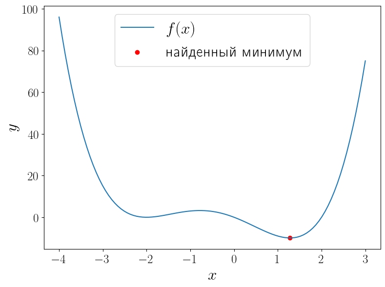
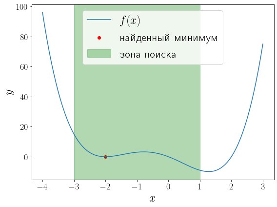
У функции (f(x) = (x – 1)x(x + 2)^2) два локальных минимума и функция minimize_scalar вернула из них глобальный. Можно сузить поиск область поиска минимума используя метод bounded.
a, b = -3, 1
solution = optimize.minimize_scalar(f, bounds=(a, b), method="bounded")

fig, ax = plt.subplots(figsize=(8, 6), layout="tight")
ax.plot(x, f(x), label="$f(x)$")
ax.scatter(solution.x, solution.fun, color="red", label="найденный минимум")
ax.set_xlabel("$x$")
ax.set_ylabel("$y$")
ax.axvspan(a, b, color="green", alpha=0.3, label="зона поиска")
ax.legend()
<matplotlib.legend.Legend at 0x1fcbc8e9e80>
Минимизация функции многих переменных#
Общий случай#
Функция scipy.optimize.minimize предназначена для минимизации функции многих переменных (fcolonmathbb{R}^ntomathbb{R}) при независимой переменной в области (Dsubsetmathbb{R}^n):
[
f(vec{x}) sim min_{vec{x}in D}.
]
При этом важно определить минимизируемую функцию именно принимающей один векторный аргумент, а не (n) скалярных.
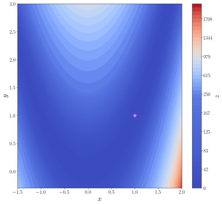
В качестве примера рассмотрим поиск минимума функции Розенброка
[
f(alpha, beta) = (1 – alpha)^2 + 100(beta – alpha^2)^2.
]
Её минимум равен 0, который достигается при (alpha = beta = 1). Для минимизации функции средствами SciPy необходимо определить её в виде функции одного векторного аргумента. Например, если положить, что (vec{x}=begin{pmatrix}x_1 \ x_2end{pmatrix}=begin{pmatrix}alpha \ betaend{pmatrix}), то функцию Розенброка можно записать в виде
[
f(vec{x}) = (1 – x_1)^2 + 100(x_2 – x_1^2)^2.
]
Именно в таком виде она уже определена в SciPy: rosen. Кроме того в SciPy доступны её градиент rosen_der и матрица Гессе rosen_hess. В ячейке ниже строится график этой функции.
import numpy as np
from scipy import optimize
from matplotlib import pyplot as plt


f = optimize.rosen


def plot_surface():
    n_points = 100
    x = np.linspace(-1.5, 2.0, n_points)
    y = np.linspace(-0.3, 3, n_points)
    xx, yy = np.meshgrid(x, y)
    X = np.vstack([xx.flatten(), yy.flatten()])
    zz = f(X).reshape(n_points, n_points)

    levels = np.hstack([np.linspace(0, 200, 25), np.linspace(250, 2000, 25)])

    fig, ax = plt.subplots(figsize=(11, 10), layout="tight")
    cf = ax.contourf(xx, yy, zz, levels=levels, cmap="coolwarm")
    cbar = fig.colorbar(cf)
    ax.set_xlabel("$x$")
    ax.set_ylabel("$y$")
    cbar.set_label("$z$")
    ax.scatter([1], [1], marker="*", s=200, color="violet", label="глобальный минимум")
    return ax

plot_surface()
<AxesSubplot:xlabel='$x$', ylabel='$y$'>
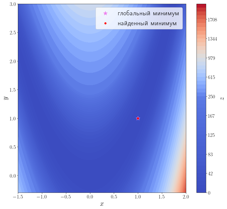
В самой простой своей форме достаточно передать методу optimize.minimize минимизируемую функцию (f) и начальное приближение (x_0).
solution = optimize.minimize(f, x0=[3, 0])
print(solution)

ax = plot_surface()
ax.scatter(solution.x[0], solution.x[1], color="red", label="найденный минимум")
ax.legend()
      fun: 2.0042284826789698e-11
 hess_inv: array([[0.49906269, 0.99813029],
       [0.99813029, 2.00126989]])
      jac: array([-2.75307058e-08,  1.52773794e-08])
  message: 'Optimization terminated successfully.'
     nfev: 168
      nit: 42
     njev: 56
   status: 0
  success: True
        x: array([0.99999552, 0.99999104])
<matplotlib.legend.Legend at 0x1fcbfe49a30>

Из возвращаемого значения видно, что метод успешно сошелся и алгоритму потребовалось 42 итерации и 168 вызовов функции f, чтобы сойтись.
Известна первая производная#
Передадим этому методу функцию, вычисляющую матрицу градиент искомой функции. Для этого необходимо использовать параметр jac этой функции.
jacobian = optimize.rosen_der

solution = optimize.minimize(f, x0=[3, 0], jac=jacobian)
print(solution)

ax = plot_surface()
ax.scatter(solution.x[0], solution.x[1], color="red", label="найденный минимум")
ax.legend()
      fun: 1.0497719786985556e-20
 hess_inv: array([[0.49999817, 1.00001013],
       [1.00001013, 2.00505181]])
      jac: array([-2.72340728e-09,  1.43485224e-09])
  message: 'Optimization terminated successfully.'
     nfev: 54
      nit: 42
     njev: 54
   status: 0
  success: True
        x: array([1., 1.])
<matplotlib.legend.Legend at 0x1fcc1803490>
Количество итераций осталось прежним, а количество вызовов функции f снизилось до 35. Это достигается за счет того, что метод минимизации вычисляет производную, вызывая переданную функцию jac, а до этого он её оценивал численно, что требовало дополнительных вызовов f.
Известны первая и вторая производные#
Передадим ещё информацию о второй производной функции f, т.е. матрицу Гессе. Метод минимизации по умолчанию (BFGS) — метод первого порядка, чтобы задействовать матрицу Гессе, необходимо использовать метод второго порядка, например, dogleg.
hessian = optimize.rosen_hess

solution = optimize.minimize(f, [3, 0], method="dogleg", jac=jacobian, hess=hessian)
print(solution)

ax = plot_surface()
ax.scatter(solution.x[0], solution.x[1], color="red", label="найденный минимум")
ax.legend()
     fun: 3.514212495812258e-16
    hess: array([[ 802.00002985, -400.00000744],
       [-400.00000744,  200.        ]])
     jac: array([ 1.31311361e-07, -4.70576911e-08])
 message: 'Optimization terminated successfully.'
    nfev: 18
    nhev: 14
     nit: 17
    njev: 15
  status: 0
 success: True
       x: array([1.00000002, 1.00000004])
<matplotlib.legend.Legend at 0x1fcbffeaa90>

Методу второго порядка потребовалось всего 17 итераций и 18 вызовов функции f, чтобы сойтись.
Время на прочтение
6 мин
Количество просмотров 31K

Задача и требования
-
Основная цель – создать алгоритм, который найдет максимальное значение по модулю минимума на заданном радиусе.
-
Алгоритм должен быть эффективным и работать достаточно быстро
-
Результат должен быть отображен на графике
Введение, описание алгоритма
Рабочая область функции (заданный интервал) разбита на несколько точек. Выбраны точки локальных минимумов. После этого все координаты передаются функции в качестве аргументов и выбирается аргумент, дающий наименьшее значение. Затем применяется метод градиентного спуска.
Реализация
Прежде всего, numpy необходим для функций sinus, cosinus и exp. Также необходимо добавить matplotlib для построения графиков.
import numpy as np
import matplotlib.pyplot as plot
Константы
radius = 8                                  # working plane radius
centre = (global_epsilon, global_epsilon)   # centre of the working circle
arr_shape = 100                             # number of points processed / 360
step = radius / arr_shape                   # step between two points
arr_shape должна быть 100, потому что, если она больше, программа начинает работать значительно медленнее. И не может быть меньше, иначе это испортит расчеты.
Функция, для которой рассчитывается минимум:
def differentiable_function(x, y):
    return np.sin(x) * np.exp((1 - np.cos(y)) ** 2) +
           np.cos(y) * np.exp((1 - np.sin(x)) ** 2) + (x - y) ** 2
Затем выбирается приращение аргумента:

Поскольку предел аргумента стремится к нулю, точность должна быть небольшой по сравнению с радиусом рабочей плоскости:
global_epsilon = 0.000000001 # argument increment for derivativeДля дальнейшего разбиения плоскости необходим поворот вектора:

Если вращение применяется к вектору (x, 0), повернутый вектор будет вычисляться следующим образом:
def rotate_vector(length, a):
    return length * np.cos(a), length * np.sin(a)
Расчет производной по оси Y, где эпсилон – значение y:
def derivative_y(epsilon, arg):
    return (differentiable_function(arg, epsilon + global_epsilon) -

        differentiable_function(arg, epsilon)) / global_epsilon
Вычисление производной по оси X, где эпсилон – значение x:
def derivative_x(epsilon, arg):
    return (differentiable_function(global_epsilon + epsilon, arg) -

         differentiable_function(epsilon, arg)) / global_epsilon
Расчет градиента:

Поскольку градиент вычисляется для 2D-функции, k равно нулю
gradient = derivative_x(x, y) + derivative_y(y, x)Схема генерации точек

Возвращаемое значение представляет собой массив приблизительных локальных минимумов.
Локальный минимум распознается по смене знака производной с минуса на плюс. Подробнее об этом здесь: https://en.wikipedia.org/wiki/Maxima_and_minima
def calculate_flip_points():
    flip_points = np.array([0, 0])
    points = np.zeros((360, arr_shape), dtype=bool)
    cx, cy = centre

    for i in range(arr_shape):
        for alpha in range(360):
            x, y = rotate_vector(step, alpha)
            x = x * i + cx
            y = y * i + cy
            points[alpha][i] = derivative_x(x, y) + derivative_y(y, x) > 0
            if not points[alpha][i - 1] and points[alpha][i]:
                flip_points = np.vstack((flip_points, np.array([alpha, i - 1])))

    return flip_points
Выбор точки из flip_points, значение функции от которой минимально:
def pick_estimates(positions):
    vx, vy = rotate_vector(step, positions[1][0])
    cx, cy = centre
    best_x, best_y = cx + vx * positions[1][1], cy + vy * positions[1][1]

    for index in range(2, len(positions)):
        vx, vy = rotate_vector(step, positions[index][0])
        x, y = cx + vx * positions[index][1], cy + vy * positions[index][1]
        if differentiable_function(best_x, best_y) > differentiable_function(x, y):
            best_x = x
            best_y = y

    for index in range(360):
        vx, vy = rotate_vector(step, index)
        x, y = cx + vx * (arr_shape - 1), cy + vy * (arr_shape - 1)
        if differentiable_function(best_x, best_y) > differentiable_function(x, y):
            best_x = x
            best_y = y

    return best_x, best_y
Метод градиентного спуска:
def gradient_descent(best_estimates, is_x):
    derivative = derivative_x if is_x else derivative_y
    best_x, best_y = best_estimates
    descent_step = step
    value = derivative(best_y, best_x)

    while abs(value) > global_epsilon:
        descent_step *= 0.95
        best_y = best_y - descent_step
            if derivative(best_y, best_x) > 0 else best_y + descent_step
        value = derivative(best_y, best_x)

    return best_y, best_x
Нахождение точки минимума:
def find_minimum():
    return gradient_descent(gradient_descent(pick_estimates(calculate_flip_points()), False), True)
Формирование сетки точек для построения:
def get_grid(grid_step):
    samples = np.arange(-radius, radius, grid_step)
    x, y = np.meshgrid(samples, samples)

return x, y, differentiable_function(x, y)
Построение графика:
def draw_chart(point, grid):
    point_x, point_y, point_z = point
    grid_x, grid_y, grid_z = grid
    plot.rcParams.update({
        'figure.figsize': (4, 4),
        'figure.dpi': 200,
        'xtick.labelsize': 4,
        'ytick.labelsize': 4
    })
    ax = plot.figure().add_subplot(111, projection='3d')
    ax.scatter(point_x, point_y, point_z, color='red')
    ax.plot_surface(grid_x, grid_y, grid_z, rstride=5, cstride=5, alpha=0.7)

plot.show()
Функция main:
if __name__ == '__main__':
    min_x, min_y = find_minimum()
    minimum = (min_x, min_y, differentiable_function(min_x, min_y))

draw_chart(minimum, get_grid(0.05))
График:

Заключение
Процесс вычисления минимального значения с помощью алгоритма может быть не очень точным при вычислениях в более крупном масштабе, например, если радиус рабочей плоскости равен 1000, но он очень быстрый по сравнению с точным. Плюс в любом случае, если радиус большой, результат находится примерно в том положении, в котором он должен быть, поэтому разница не будет заметна на графике.
Исходный код:
import numpy as np
import matplotlib.pyplot as plot


radius = 8                                  # working plane radius
global_epsilon = 0.000000001                # argument increment for derivative
centre = (global_epsilon, global_epsilon)   # centre of the working circle
arr_shape = 100                             # number of points processed / 360
step = radius / arr_shape                   # step between two points


def differentiable_function(x, y):
    return np.sin(x) * np.exp((1 - np.cos(y)) ** 2) +
           np.cos(y) * np.exp((1 - np.sin(x)) ** 2) + (x - y) ** 2


def rotate_vector(length, a):
    return length * np.cos(a), length * np.sin(a)


def derivative_x(epsilon, arg):
    return (differentiable_function(global_epsilon + epsilon, arg) -
            differentiable_function(epsilon, arg)) / global_epsilon


def derivative_y(epsilon, arg):
    return (differentiable_function(arg, epsilon + global_epsilon) -
            differentiable_function(arg, epsilon)) / global_epsilon


def calculate_flip_points():
    flip_points = np.array([0, 0])
    points = np.zeros((360, arr_shape), dtype=bool)
    cx, cy = centre

    for i in range(arr_shape):
        for alpha in range(360):
            x, y = rotate_vector(step, alpha)
            x = x * i + cx
            y = y * i + cy
            points[alpha][i] = derivative_x(x, y) + derivative_y(y, x) > 0
            if not points[alpha][i - 1] and points[alpha][i]:
                flip_points = np.vstack((flip_points, np.array([alpha, i - 1])))

    return flip_points


def pick_estimates(positions):
    vx, vy = rotate_vector(step, positions[1][0])
    cx, cy = centre
    best_x, best_y = cx + vx * positions[1][1], cy + vy * positions[1][1]

    for index in range(2, len(positions)):
        vx, vy = rotate_vector(step, positions[index][0])
        x, y = cx + vx * positions[index][1], cy + vy * positions[index][1]
        if differentiable_function(best_x, best_y) > differentiable_function(x, y):
            best_x = x
            best_y = y

    for index in range(360):
        vx, vy = rotate_vector(step, index)
        x, y = cx + vx * (arr_shape - 1), cy + vy * (arr_shape - 1)
        if differentiable_function(best_x, best_y) > differentiable_function(x, y):
            best_x = x
            best_y = y

    return best_x, best_y


def gradient_descent(best_estimates, is_x):
    derivative = derivative_x if is_x else derivative_y
    best_x, best_y = best_estimates
    descent_step = step
    value = derivative(best_y, best_x)

    while abs(value) > global_epsilon:
        descent_step *= 0.95
        best_y = best_y - descent_step
            if derivative(best_y, best_x) > 0 else best_y + descent_step
        value = derivative(best_y, best_x)

    return best_y, best_x


def find_minimum():
    return gradient_descent(gradient_descent(pick_estimates(calculate_flip_points()), False), True)


def get_grid(grid_step):
    samples = np.arange(-radius, radius, grid_step)
    x, y = np.meshgrid(samples, samples)
    return x, y, differentiable_function(x, y)


def draw_chart(point, grid):
    point_x, point_y, point_z = point
    grid_x, grid_y, grid_z = grid
    plot.rcParams.update({
        'figure.figsize': (4, 4),
        'figure.dpi': 200,
        'xtick.labelsize': 4,
        'ytick.labelsize': 4
    })
    ax = plot.figure().add_subplot(111, projection='3d')
    ax.scatter(point_x, point_y, point_z, color='red')
    ax.plot_surface(grid_x, grid_y, grid_z, rstride=5, cstride=5, alpha=0.7)
    plot.show()


if __name__ == '__main__':
    min_x, min_y = find_minimum()
    minimum = (min_x, min_y, differentiable_function(min_x, min_y))
    draw_chart(minimum, get_grid(0.05))