Using, for instance, scipy‘s fmin (which contains an implementation of the Nelder-Mead algorithm), you can try this:
import numpy as np
from scipy.optimize import fmin
import math

def f(x):
    exp = (math.pow(x[0], 2) + math.pow(x[1], 2)) * -1
    return math.exp(exp) * math.cos(x[0] * x[1]) * math.sin(x[0] * x[1])

fmin(f,np.array([0,0]))
which yields the following output:
Optimization terminated successfully.
     Current function value: -0.161198
     Iterations: 60
     Function evaluations: 113
array([ 0.62665701, -0.62663095])
Please keep in mind that:
1) with scipy you need to convert your function into a function accepting an array (I showed how to do it in the example above);
2) fmin uses, like most of its pairs, an iterative algorithm, therefore you must provide a starting point (in my example, I provided (0,0)). You can provide different starting points to obtain different minima/maxima.
Поиск минимума#
Подмодуль scipy.optimize содержит в себе множество методов для решения задач оптимизации (минимизация, максимизация).
from matplotlib import pyplot as plt


def configure_matplotlib():
    plt.rc('text', usetex=True)
    plt.rcParams["axes.titlesize"] = 28
    plt.rcParams["axes.labelsize"] = 24
    plt.rcParams["legend.fontsize"] = 24
    plt.rcParams["xtick.labelsize"] = plt.rcParams["ytick.labelsize"] = 18
    plt.rcParams["text.latex.preamble"] = r"""
    usepackage[utf8]{inputenc}
    usepackage[english,russian]{babel}
    usepackage{amsmath}
    """

configure_matplotlib()
Минимизация скалярной функции одного аргумента#
Функция scipy.optimize.minimize_scalar ищет минимум функции (fcolon mathbb{R} to mathbb{R}) при независимой переменной в области (Dsubsetmathbb{R}), т.е. решает задачу
[
f(x) sim min_{x in D},
]
иными словами задачу поиска (x^*inmathbb{R}), такого что
[
f(x^*) = minlimits_{xin D} f(x).
]
import numpy as np
from scipy import optimize
from matplotlib import pyplot as plt


def f(x):
    return (x - 2) * x * (x + 2)**2


solution = optimize.minimize_scalar(f)
print(solution)


x = np.linspace(-4, 3, 100)

fig, ax = plt.subplots(figsize=(8, 6), layout="tight")
ax.plot(x, f(x), label=r"$f(x)$")
ax.scatter(solution.x, solution.fun, color="red", label="найденный минимум")
ax.set_xlabel("$x$")
ax.set_ylabel("$y$")
ax.legend()
     fun: -9.914949590828147
 message: 'nOptimization terminated successfully;nThe returned value satisfies the termination criterian(using xtol = 1.48e-08 )'
    nfev: 15
     nit: 11
 success: True
       x: 1.2807764040333458
<matplotlib.legend.Legend at 0x2a85390ec50>
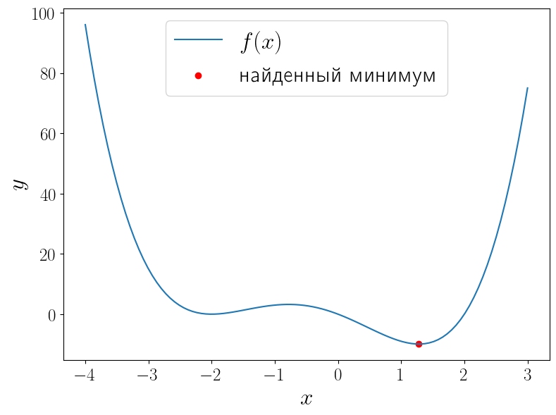
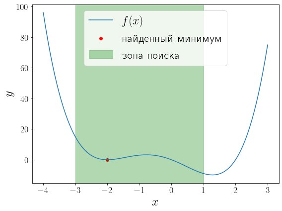
У функции (f(x) = (x – 1)x(x + 2)^2) два локальных минимума и функция minimize_scalar вернула из них глобальный. Можно сузить поиск область поиска минимума используя метод bounded.
a, b = -3, 1
solution = optimize.minimize_scalar(f, bounds=(a, b), method="bounded")

fig, ax = plt.subplots(figsize=(8, 6), layout="tight")
ax.plot(x, f(x), label="$f(x)$")
ax.scatter(solution.x, solution.fun, color="red", label="найденный минимум")
ax.set_xlabel("$x$")
ax.set_ylabel("$y$")
ax.axvspan(a, b, color="green", alpha=0.3, label="зона поиска")
ax.legend()
<matplotlib.legend.Legend at 0x1fcbc8e9e80>
Минимизация функции многих переменных#
Общий случай#
Функция scipy.optimize.minimize предназначена для минимизации функции многих переменных (fcolonmathbb{R}^ntomathbb{R}) при независимой переменной в области (Dsubsetmathbb{R}^n):
[
f(vec{x}) sim min_{vec{x}in D}.
]
При этом важно определить минимизируемую функцию именно принимающей один векторный аргумент, а не (n) скалярных.
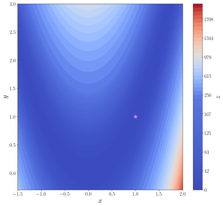
В качестве примера рассмотрим поиск минимума функции Розенброка
[
f(alpha, beta) = (1 – alpha)^2 + 100(beta – alpha^2)^2.
]
Её минимум равен 0, который достигается при (alpha = beta = 1). Для минимизации функции средствами SciPy необходимо определить её в виде функции одного векторного аргумента. Например, если положить, что (vec{x}=begin{pmatrix}x_1 \ x_2end{pmatrix}=begin{pmatrix}alpha \ betaend{pmatrix}), то функцию Розенброка можно записать в виде
[
f(vec{x}) = (1 – x_1)^2 + 100(x_2 – x_1^2)^2.
]
Именно в таком виде она уже определена в SciPy: rosen. Кроме того в SciPy доступны её градиент rosen_der и матрица Гессе rosen_hess. В ячейке ниже строится график этой функции.
import numpy as np
from scipy import optimize
from matplotlib import pyplot as plt


f = optimize.rosen


def plot_surface():
    n_points = 100
    x = np.linspace(-1.5, 2.0, n_points)
    y = np.linspace(-0.3, 3, n_points)
    xx, yy = np.meshgrid(x, y)
    X = np.vstack([xx.flatten(), yy.flatten()])
    zz = f(X).reshape(n_points, n_points)

    levels = np.hstack([np.linspace(0, 200, 25), np.linspace(250, 2000, 25)])

    fig, ax = plt.subplots(figsize=(11, 10), layout="tight")
    cf = ax.contourf(xx, yy, zz, levels=levels, cmap="coolwarm")
    cbar = fig.colorbar(cf)
    ax.set_xlabel("$x$")
    ax.set_ylabel("$y$")
    cbar.set_label("$z$")
    ax.scatter([1], [1], marker="*", s=200, color="violet", label="глобальный минимум")
    return ax

plot_surface()
<AxesSubplot:xlabel='$x$', ylabel='$y$'>
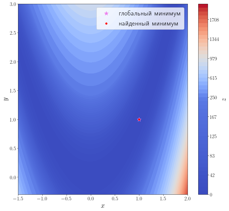
В самой простой своей форме достаточно передать методу optimize.minimize минимизируемую функцию (f) и начальное приближение (x_0).
solution = optimize.minimize(f, x0=[3, 0])
print(solution)

ax = plot_surface()
ax.scatter(solution.x[0], solution.x[1], color="red", label="найденный минимум")
ax.legend()
      fun: 2.0042284826789698e-11
 hess_inv: array([[0.49906269, 0.99813029],
       [0.99813029, 2.00126989]])
      jac: array([-2.75307058e-08,  1.52773794e-08])
  message: 'Optimization terminated successfully.'
     nfev: 168
      nit: 42
     njev: 56
   status: 0
  success: True
        x: array([0.99999552, 0.99999104])
<matplotlib.legend.Legend at 0x1fcbfe49a30>

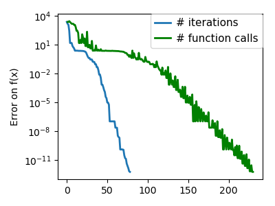
Из возвращаемого значения видно, что метод успешно сошелся и алгоритму потребовалось 42 итерации и 168 вызовов функции f, чтобы сойтись.
Известна первая производная#
Передадим этому методу функцию, вычисляющую матрицу градиент искомой функции. Для этого необходимо использовать параметр jac этой функции.
jacobian = optimize.rosen_der

solution = optimize.minimize(f, x0=[3, 0], jac=jacobian)
print(solution)

ax = plot_surface()
ax.scatter(solution.x[0], solution.x[1], color="red", label="найденный минимум")
ax.legend()
      fun: 1.0497719786985556e-20
 hess_inv: array([[0.49999817, 1.00001013],
       [1.00001013, 2.00505181]])
      jac: array([-2.72340728e-09,  1.43485224e-09])
  message: 'Optimization terminated successfully.'
     nfev: 54
      nit: 42
     njev: 54
   status: 0
  success: True
        x: array([1., 1.])
<matplotlib.legend.Legend at 0x1fcc1803490>
Количество итераций осталось прежним, а количество вызовов функции f снизилось до 35. Это достигается за счет того, что метод минимизации вычисляет производную, вызывая переданную функцию jac, а до этого он её оценивал численно, что требовало дополнительных вызовов f.
Известны первая и вторая производные#
Передадим ещё информацию о второй производной функции f, т.е. матрицу Гессе. Метод минимизации по умолчанию (BFGS) — метод первого порядка, чтобы задействовать матрицу Гессе, необходимо использовать метод второго порядка, например, dogleg.
hessian = optimize.rosen_hess

solution = optimize.minimize(f, [3, 0], method="dogleg", jac=jacobian, hess=hessian)
print(solution)

ax = plot_surface()
ax.scatter(solution.x[0], solution.x[1], color="red", label="найденный минимум")
ax.legend()
     fun: 3.514212495812258e-16
    hess: array([[ 802.00002985, -400.00000744],
       [-400.00000744,  200.        ]])
     jac: array([ 1.31311361e-07, -4.70576911e-08])
 message: 'Optimization terminated successfully.'
    nfev: 18
    nhev: 14
     nit: 17
    njev: 15
  status: 0
 success: True
       x: array([1.00000002, 1.00000004])
<matplotlib.legend.Legend at 0x1fcbffeaa90>

Методу второго порядка потребовалось всего 17 итераций и 18 вызовов функции f, чтобы сойтись.
Время на прочтение
5 мин
Количество просмотров 56K
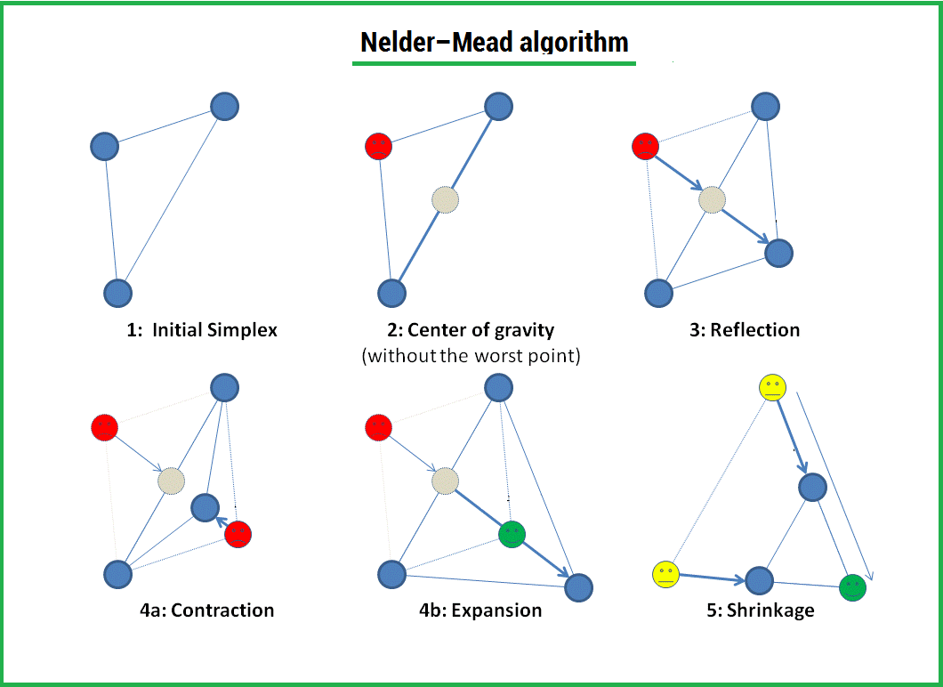
Метод Нелдера — Мида — метод оптимизации (поиска минимума) функции от нескольких переменных. Простой и в тоже время эффективный метод, позволяющий оптимизировать функции без использования градиентов. Метод надежен и, как правило, показывает хорошие результаты, хотя и отсутствует теория сходимости. Может использоваться в функции optimize из модуля scipy.optimize популярной библиотеки для языка python, которая используется для математических расчетов.
Алгоритм заключается в формировании симплекса (simplex) и последующего его деформирования в направлении минимума, посредством трех операций:
1) Отражение (reflection);
2) Растяжение (expansion);
3) Сжатие (contract);
Симплекс представляет из себя геометрическую фигуру, являющуюся n — мерным обобщением треугольника. Для одномерного пространства — это отрезок, для двумерного — треугольник. Таким образом n — мерный симплекс имеет n + 1 вершину.
Алгоритм
1) Пусть
 функция, которую необходимо оптимизировать. На первом шаге выбираем три случайные точки (об этом чуть позже) и формируем симплекс (треугольник). Вычисляем значение функции в каждой точке:
 ,
,
 ,
,
 .
.
Сортируем точки по значениям функции
в этих точках, таким образом получаем двойное неравенство:

Мы ищем минимум функции, а следовательно, на данном шаге лучшей будет та точка, в которой значение функции минимально. Для удобства переобозначим точки следующим образом:
b =
 , g =
, g =
 , w =
, w =
 , где best, good, worst — соответственно.
2) На следующем шаге находим середину отрезка, точками которого являются g и b. Т.к. координаты середины отрезка равны полусумме координат его концов, получаем:

В более общем виде можно записать так:

3) Применяем операцию отражения:
Находим точку
 , следующим образом:

Т.е. фактически отражаем точку w относительно mid. В качестве коэффициента берут как правило 1. Проверяем нашу точку: если
 , то это хорошая точка. А теперь попробуем расстояние увеличить в 2 раза, вдруг нам повезет и мы найдем точку еще лучше.
4) Применяем операцию растяжения:
Находим точку
 следующим образом:

В качестве γ принимаем γ = 2, т.е. расстояние увеличиваем в 2 раза.
Проверяем точку
:
Если
 , то нам повезло и мы нашли точку лучше, чем есть на данный момент, если бы этого не произошло, мы бы остановились на точке
.
Далее заменяем точку w на
, в итоге получаем:
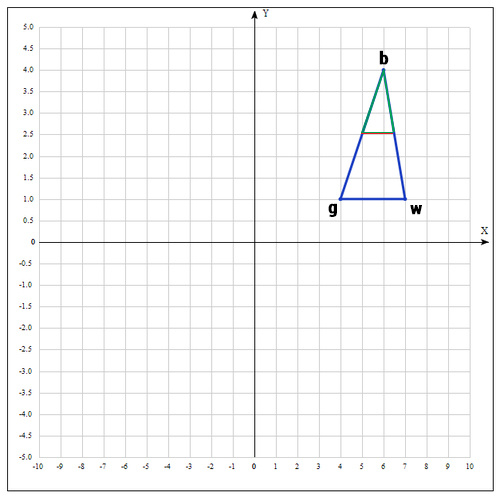
5) Если же нам совсем не повезло и мы не нашли хороших точек, пробуем операцию сжатия.
Как следует из названия операции мы будем уменьшать наш отрезок и искать хорошие точки внутри треугольника.
Пробуем найти хорошую точку
 :
:

Коэффициент β принимаем равным 0.5, т.е. точка
на середине отрезка wmid.
Существует еще одна операция — shrink (сокращение). В данном случае, мы переопределяем весь симплекс. Оставляем только «лучшую» точку, остальные определяем следующим образом:

Коэффициент δ берут равным 0.5.
По существу передвигаем точки по направлению к текущей «лучшей» точке. Преобразование выглядит следующим образом:
Необходимо отметить, что данная операция дорого обходится, поскольку необходимо заменять точки в симплексе. К счастью было установлено, при проведении большого количества экспериментов, что shrink — трансформация редко случается на практике.
Алгоритм заканчивается, когда:
1) Было выполнено необходимое количество итераций.
2) Площадь симплекса достигла определенной величины.
3) Текущее лучшее решение достигло необходимой точности.
Как и в большинстве эвристических методов, не существует идеального способа выбора инициализирующих точек. Как уже было сказано, можно брать случайные точки, находящиеся недалеко друг от друга для формирования симплекса; но есть решение и получше, которое используется в реализации алгоритма в MATHLAB:
Выбор первой точки
поручаем пользователю, если он имеет некоторое представление о возможном хорошем решении, в противном случае выбирается случайным образом. Остальные точки выбираются исходя из
, на небольшом расстоянии вдоль направления каждого измерения:

где
 — единичный вектор.
 определяется таким образом:
= 0.05, если коэффициент при
в определении
не нулевой.
= 0.00025, если коэффициент при
в определении нулевой.
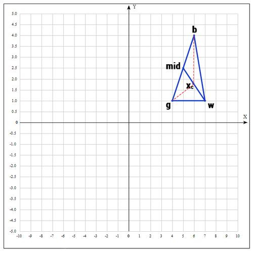
Пример:
Найти экстремум следующей функции:

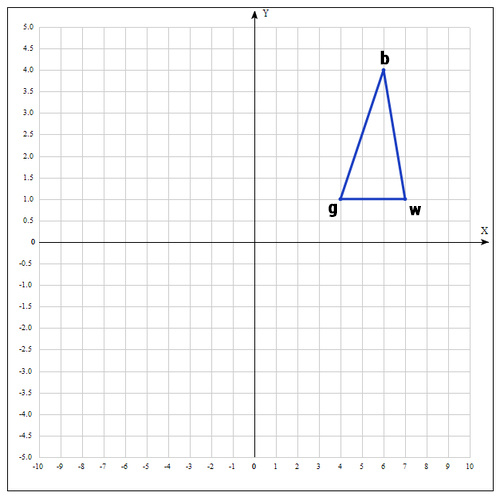
В качестве начальных возьмем точки:

Вычислим значение функции в каждой точке:


Переобозначим точки следующим образом:

Находим середину отрезка bg:

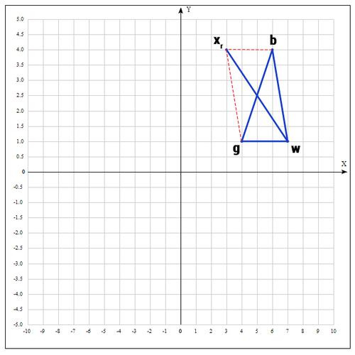
Находим точку
(операция отражения):

если α=1, тогда:

Проверяем точку
:
 , т.к.
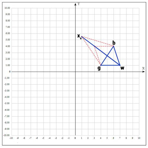
 пробуем увеличить отрезок (операция растяжения).

если γ = 2, тогда:


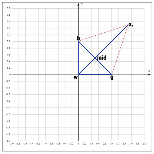
Проверяем значение функции в точке
:

Оказалось, что точка
«лучше» точки b. Следовательно мы получаем новые вершины:

И алгоритм начинается сначала.
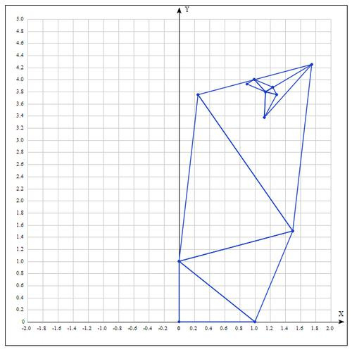
Таблица значений для 10 итераций:
| Best | Good | Worst |
|---|---|---|
 |
 |
 |
 |
|
|
 |
|
|
|
 |
|
 |
|
 |
 |
 |
|
|
 |
|
|
 |
|
 |
|
 |
|
 |
|
Аналитически находим экстремум функции, он достигается в точке
 .
.
После 10 итераций мы получаем достаточно точное приближение:

Еще о методе:
Алгоритм Нелдера — Мида в основном используется для выбора параметра в машинном обучении. В сущности, симплекс-метод используется для оптимизации параметров модели. Это связано с тем, что данный метод оптимизирует целевую функцию довольно быстро и эффективно (особенно там, где не используется shrink — модификация).
С другой стороны, в силу отсутствия теории сходимости, на практике метод может приводить к неверному ответу даже на гладких (непрерывно дифференцируемых) функциях. Также возможна ситуация, когда рабочий симплекс находится далеко от оптимальной точки, а алгоритм производит большое число итераций, при этом мало изменяя значения функции. Эвристический метод решения этой проблемы заключается в запуске алгоритма несколько раз и ограничении числа итераций.
Реализация на языке программирования python:
Создаем вспомогательный класс Vector и перегружаем операторы для возможности производить с векторами базовые операции. Я намерено не использовал вспомогательные библиотеки для реализации алгоритма, т.к. в таком случае зачастую снижается восприятие.
#!/usr/bin/python
# -*- coding: utf-8 -*-
class Vector(object):
def __init__(self, x, y):
""" Create a vector, example: v = Vector(1,2) """
self.x = x
self.y = y
def __repr__(self):
return "({0}, {1})".format(self.x, self.y)
def __add__(self, other):
x = self.x + other.x
y = self.y + other.y
return Vector(x, y)
def __sub__(self, other):
x = self.x - other.x
y = self.y - other.y
return Vector(x, y)
def __rmul__(self, other):
x = self.x * other
y = self.y * other
return Vector(x, y)
def __truediv__(self, other):
x = self.x / other
y = self.y / other
return Vector(x, y)
def c(self):
return (self.x, self.y)
# objective function
def f(point):
x, y = point
return x**2 + x*y + y**2 - 6*x - 9*y
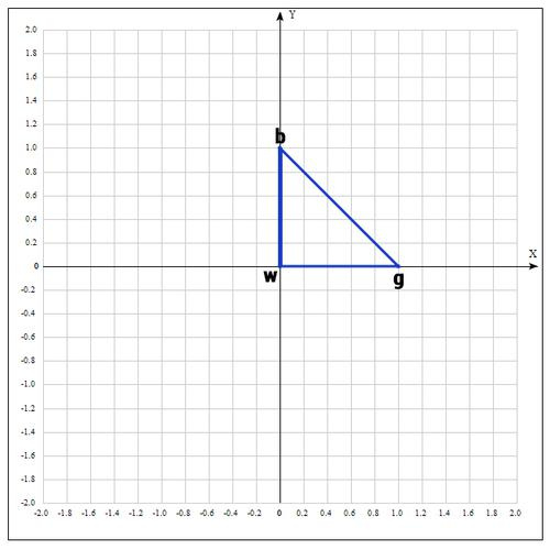
def nelder_mead(alpha=1, beta=0.5, gamma=2, maxiter=10):
# initialization
v1 = Vector(0, 0)
v2 = Vector(1.0, 0)
v3 = Vector(0, 1)
for i in range(maxiter):
adict = {v1:f(v1.c()), v2:f(v2.c()), v3:f(v3.c())}
points = sorted(adict.items(), key=lambda x: x[1])
b = points[0][0]
g = points[1][0]
w = points[2][0]
mid = (g + b)/2
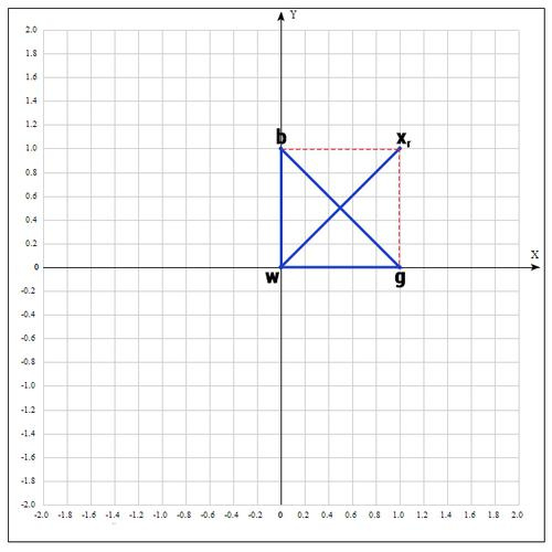
# reflection
xr = mid + alpha * (mid - w)
if f(xr.c()) < f(g.c()):
w = xr
else:
if f(xr.c()) < f(w.c()):
w = xr
c = (w + mid)/2
if f(c.c()) < f(w.c()):
w = c
if f(xr.c()) < f(b.c()):
# expansion
xe = mid + gamma * (xr - mid)
if f(xe.c()) < f(xr.c()):
w = xe
else:
w = xr
if f(xr.c()) > f(g.c()):
# contraction
xc = mid + beta * (w - mid)
if f(xc.c()) < f(w.c()):
w = xc
# update points
v1 = w
v2 = g
v3 = b
return b
print("Result of Nelder-Mead algorithm: ")
xk = nelder_mead()
print("Best poits is: %s"%(xk))
Спасибо за чтение статьи. Надеюсь она была Вам полезна и Вы узнали много нового.
С вами был FUNNYDMAN. Удачной оптимизации!)
2.7. Mathematical optimization: finding minima of functions
Authors: Gaël Varoquaux
Mathematical optimization deals with the
problem of finding numerically minimums (or maximums or zeros) of
a function. In this context, the function is called cost function, or
objective function, or energy.
Here, we are interested in using scipy.optimize for black-box
optimization: we do not rely on the mathematical expression of the
function that we are optimizing. Note that this expression can often be
used for more efficient, non black-box, optimization.
See also
References
Mathematical optimization is very … mathematical. If you want
performance, it really pays to read the books:
- Convex Optimization
by Boyd and Vandenberghe (pdf available free online). - Numerical Optimization,
by Nocedal and Wright. Detailed reference on gradient descent methods. - Practical Methods of Optimization by Fletcher: good at hand-waving explanations.
Chapters contents
- Knowing your problem
- Convex versus non-convex optimization
- Smooth and non-smooth problems
- Noisy versus exact cost functions
- Constraints
- A review of the different optimizers
- Getting started: 1D optimization
- Gradient based methods
- Newton and quasi-newton methods
- Full code examples
- Examples for the mathematical optimization chapter
- Gradient-less methods
- Global optimizers
- Practical guide to optimization with scipy
- Choosing a method
- Making your optimizer faster
- Computing gradients
- Synthetic exercices
- Special case: non-linear least-squares
- Minimizing the norm of a vector function
- Curve fitting
- Optimization with constraints
- Box bounds
- General constraints
- Full code examples
- Examples for the mathematical optimization chapter
2.7.1. Knowing your problem
Not all optimization problems are equal. Knowing your problem enables you
to choose the right tool.
Dimensionality of the problem
The scale of an optimization problem is pretty much set by the
dimensionality of the problem, i.e. the number of scalar variables
on which the search is performed.
2.7.1.1. Convex versus non-convex optimization
 |
 |
|
A convex function:
|
A non-convex function |
Optimizing convex functions is easy. Optimizing non-convex functions can
be very hard.
Note
It can be proven that for a convex function a local minimum is
also a global minimum. Then, in some sense, the minimum is unique.
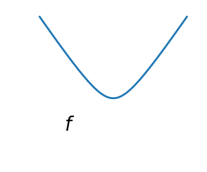
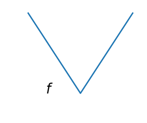
2.7.1.2. Smooth and non-smooth problems
 |
 |
|
A smooth function: The gradient is defined everywhere, and is a continuous function |
A non-smooth function |
Optimizing smooth functions is easier
(true in the context of black-box optimization, otherwise
Linear Programming
is an example of methods which deal very efficiently with
piece-wise linear functions).
2.7.1.3. Noisy versus exact cost functions
| Noisy (blue) and non-noisy (green) functions | 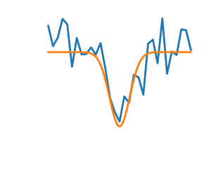 |
Noisy gradients
Many optimization methods rely on gradients of the objective function.
If the gradient function is not given, they are computed numerically,
which induces errors. In such situation, even if the objective
function is not noisy, a gradient-based optimization may be a noisy
optimization.
2.7.1.4. Constraints
|
Optimizations under constraints Here:
|
 |
2.7.2. A review of the different optimizers
2.7.2.1. Getting started: 1D optimization
Let’s get started by finding the minimum of the scalar function
![f(x)=exp[(x-0.7)^2]](https://scipy-lectures.org/_images/math/c8b2b4fa34dbb68f7c75a530d0fc24e3c4a6c6f1.png) .
. scipy.optimize.minimize_scalar() uses
Brent’s method to find the minimum of a function:
>>> from scipy import optimize
>>> def f(x):
...     return -np.exp(-(x - 0.7)**2)
>>> result = optimize.minimize_scalar(f)
>>> result.success # check if solver was successful
True
>>> x_min = result.x
>>> x_min
0.699999999...
>>> x_min - 0.7
-2.16...e-10
| Brent’s method on a quadratic function: it converges in 3 iterations, as the quadratic approximation is then exact. |
 |
 |
| Brent’s method on a non-convex function: note that the fact that the optimizer avoided the local minimum is a matter of luck. |
 |
 |
Note
You can use different solvers using the parameter method.
2.7.2.2. Gradient based methods
Some intuitions about gradient descent
Here we focus on intuitions, not code. Code will follow.
Gradient descent
basically consists in taking small steps in the direction of the
gradient, that is the direction of the steepest descent.
| A well-conditioned quadratic function. | 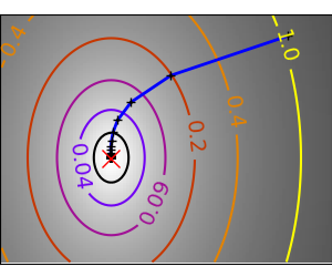 |
 |
|
An ill-conditioned quadratic function. The core problem of gradient-methods on ill-conditioned problems is |
 |
 |
We can see that very anisotropic (ill-conditioned) functions are harder
to optimize.
Take home message: conditioning number and preconditioning
If you know natural scaling for your variables, prescale them so that
they behave similarly. This is related to preconditioning.
Also, it clearly can be advantageous to take bigger steps. This
is done in gradient descent code using a
line search.
| A well-conditioned quadratic function. | 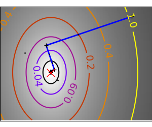 |
 |
| An ill-conditioned quadratic function. | 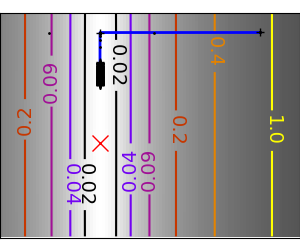 |
 |
| An ill-conditioned non-quadratic function. | 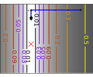 |
 |
| An ill-conditioned very non-quadratic function. | 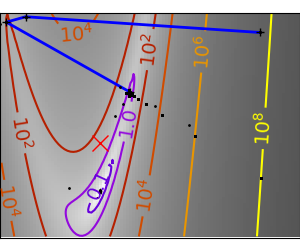 |
 |
The more a function looks like a quadratic function (elliptic
iso-curves), the easier it is to optimize.
Conjugate gradient descent
The gradient descent algorithms above are toys not to be used on real
problems.
As can be seen from the above experiments, one of the problems of the
simple gradient descent algorithms, is that it tends to oscillate across
a valley, each time following the direction of the gradient, that makes
it cross the valley. The conjugate gradient solves this problem by adding
a friction term: each step depends on the two last values of the
gradient and sharp turns are reduced.
| An ill-conditioned non-quadratic function. | 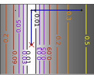 |
 |
| An ill-conditioned very non-quadratic function. | 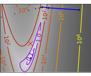 |
 |
scipy provides scipy.optimize.minimize() to find the minimum of scalar
functions of one or more variables. The simple conjugate gradient method can
be used by setting the parameter method to CG
>>> def f(x):   # The rosenbrock function
...     return .5*(1 - x[0])**2 + (x[1] - x[0]**2)**2
>>> optimize.minimize(f, [2, -1], method="CG")
     fun: 1.6...e-11
     jac: array([-6.15...e-06,   2.53...e-07])
 message: ...'Optimization terminated successfully.'
    nfev: 108
     nit: 13
    njev: 27
  status: 0
 success: True
       x: array([0.99999...,  0.99998...])
Gradient methods need the Jacobian (gradient) of the function. They can compute it
numerically, but will perform better if you can pass them the gradient:
>>> def jacobian(x):
...     return np.array((-2*.5*(1 - x[0]) - 4*x[0]*(x[1] - x[0]**2), 2*(x[1] - x[0]**2)))
>>> optimize.minimize(f, [2, 1], method="CG", jac=jacobian)
     fun: 2.957...e-14
     jac: array([ 7.1825...e-07,  -2.9903...e-07])
 message: 'Optimization terminated successfully.'
    nfev: 16
     nit: 8
    njev: 16
  status: 0
 success: True
       x: array([1.0000...,  1.0000...])
Note that the function has only been evaluated 27 times, compared to 108
without the gradient.
2.7.2.3. Newton and quasi-newton methods
Newton methods: using the Hessian (2nd differential)
Newton methods use a
local quadratic approximation to compute the jump direction. For this
purpose, they rely on the 2 first derivative of the function: the
gradient and the Hessian.
|
An ill-conditioned quadratic function: Note that, as the quadratic approximation is exact, the Newton |
 |
 |
|
An ill-conditioned non-quadratic function: Here we are optimizing a Gaussian, which is always below its |
 |
 |
| An ill-conditioned very non-quadratic function: | 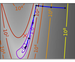 |
 |
In scipy, you can use the Newton method by setting method to Newton-CG in
scipy.optimize.minimize(). Here, CG refers to the fact that an internal
inversion of the Hessian is performed by conjugate gradient
>>> def f(x):   # The rosenbrock function
...     return .5*(1 - x[0])**2 + (x[1] - x[0]**2)**2
>>> def jacobian(x):
...     return np.array((-2*.5*(1 - x[0]) - 4*x[0]*(x[1] - x[0]**2), 2*(x[1] - x[0]**2)))
>>> optimize.minimize(f, [2,-1], method="Newton-CG", jac=jacobian)
     fun: 1.5...e-15
     jac: array([  1.0575...e-07,  -7.4832...e-08])
 message: ...'Optimization terminated successfully.'
    nfev: 11
    nhev: 0
     nit: 10
    njev: 52
  status: 0
 success: True
       x: array([0.99999...,  0.99999...])
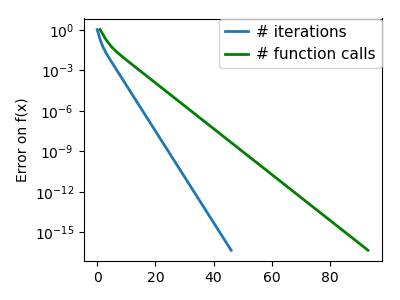
Note that compared to a conjugate gradient (above), Newton’s method has
required less function evaluations, but more gradient evaluations, as it
uses it to approximate the Hessian. Let’s compute the Hessian and pass it
to the algorithm:
>>> def hessian(x): # Computed with sympy
...     return np.array(((1 - 4*x[1] + 12*x[0]**2, -4*x[0]), (-4*x[0], 2)))
>>> optimize.minimize(f, [2,-1], method="Newton-CG", jac=jacobian, hess=hessian)
     fun: 1.6277...e-15
     jac: array([  1.1104...e-07,  -7.7809...e-08])
 message: ...'Optimization terminated successfully.'
    nfev: 11
    nhev: 10
     nit: 10
    njev: 20
  status: 0
 success: True
       x: array([0.99999...,  0.99999...])
Note
At very high-dimension, the inversion of the Hessian can be costly
and unstable (large scale > 250).
Note
Newton optimizers should not to be confused with Newton’s root finding
method, based on the same principles, scipy.optimize.newton().
Quasi-Newton methods: approximating the Hessian on the fly
BFGS: BFGS (Broyden-Fletcher-Goldfarb-Shanno algorithm) refines at
each step an approximation of the Hessian.
2.7.3. Full code examples
2.7.4. Examples for the mathematical optimization chapter
Gallery generated by Sphinx-Gallery
|
An ill-conditioned quadratic function: On a exactly quadratic function, BFGS is not as fast as Newton’s |
 |
 |
|
An ill-conditioned non-quadratic function: Here BFGS does better than Newton, as its empirical estimate of the |
 |
 |
| An ill-conditioned very non-quadratic function: | 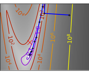 |
 |
>>> def f(x):   # The rosenbrock function
...     return .5*(1 - x[0])**2 + (x[1] - x[0]**2)**2
>>> def jacobian(x):
...     return np.array((-2*.5*(1 - x[0]) - 4*x[0]*(x[1] - x[0]**2), 2*(x[1] - x[0]**2)))
>>> optimize.minimize(f, [2, -1], method="BFGS", jac=jacobian)
      fun: 2.6306...e-16
 hess_inv: array([[0.99986...,  2.0000...],
       [2.0000...,  4.498...]])
      jac: array([  6.7089...e-08,  -3.2222...e-08])
  message: ...'Optimization terminated successfully.'
     nfev: 10
      nit: 8
     njev: 10
   status: 0
  success: True
        x: array([1.        ,  0.99999...])
L-BFGS: Limited-memory BFGS Sits between BFGS and conjugate gradient:
in very high dimensions (> 250) the Hessian matrix is too costly to
compute and invert. L-BFGS keeps a low-rank version. In addition, box bounds
are also supported by L-BFGS-B:
>>> def f(x):   # The rosenbrock function
...     return .5*(1 - x[0])**2 + (x[1] - x[0]**2)**2
>>> def jacobian(x):
...     return np.array((-2*.5*(1 - x[0]) - 4*x[0]*(x[1] - x[0]**2), 2*(x[1] - x[0]**2)))
>>> optimize.minimize(f, [2, 2], method="L-BFGS-B", jac=jacobian)
      fun: 1.4417...e-15
 hess_inv: <2x2 LbfgsInvHessProduct with dtype=float64>
      jac: array([  1.0233...e-07,  -2.5929...e-08])
  message: ...'CONVERGENCE: NORM_OF_PROJECTED_GRADIENT_<=_PGTOL'
     nfev: 17
      nit: 16
   status: 0
  success: True
        x: array([1.0000...,  1.0000...])
2.7.4.12. Gradient-less methods
A shooting method: the Powell algorithm
Almost a gradient approach
|
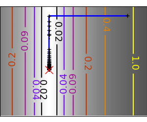
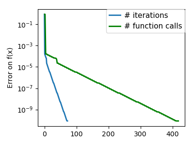
An ill-conditioned quadratic function: Powell’s method isn’t too sensitive to local ill-conditionning in |
 |
 |
| An ill-conditioned very non-quadratic function: | 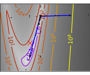 |
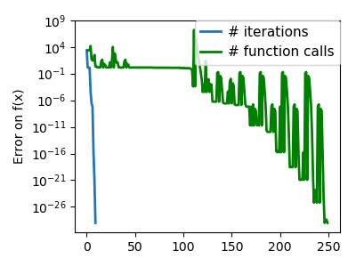 |
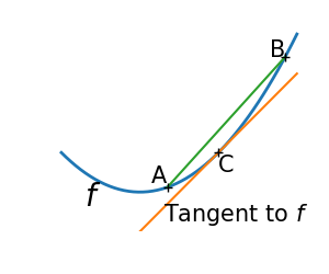
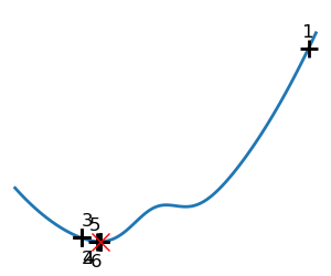
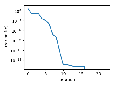
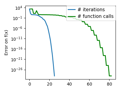
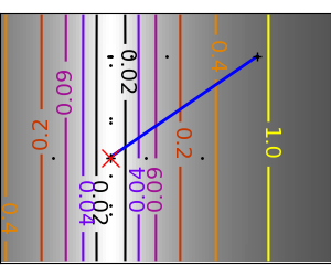
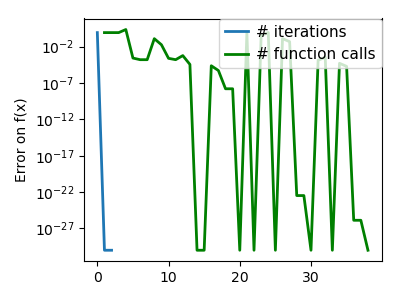
Simplex method: the Nelder-Mead
The Nelder-Mead algorithms is a generalization of dichotomy approaches to
high-dimensional spaces. The algorithm works by refining a simplex, the generalization of intervals
and triangles to high-dimensional spaces, to bracket the minimum.
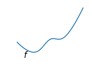
Strong points: it is robust to noise, as it does not rely on
computing gradients. Thus it can work on functions that are not locally
smooth such as experimental data points, as long as they display a
large-scale bell-shape behavior. However it is slower than gradient-based
methods on smooth, non-noisy functions.
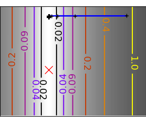
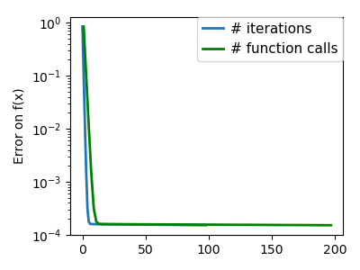
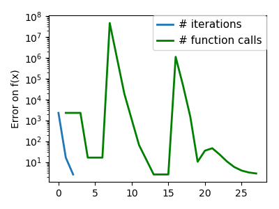
| An ill-conditioned non-quadratic function: |  |
 |
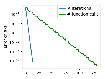
| An ill-conditioned very non-quadratic function: | 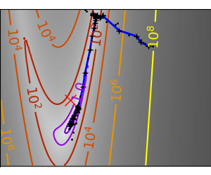 |
 |
Using the Nelder-Mead solver in scipy.optimize.minimize():
>>> def f(x):   # The rosenbrock function
...     return .5*(1 - x[0])**2 + (x[1] - x[0]**2)**2
>>> optimize.minimize(f, [2, -1], method="Nelder-Mead")
 final_simplex: (array([[1.0000...,  1.0000...],
       [0.99998... ,  0.99996... ],
       [1.0000...,  1.0000... ]]), array([1.1152...e-10,   1.5367...e-10,   4.9883...e-10]))
           fun: 1.1152...e-10
       message: ...'Optimization terminated successfully.'
          nfev: 111
           nit: 58
        status: 0
       success: True
             x: array([1.0000...,  1.0000...])
2.7.4.13. Global optimizers
If your problem does not admit a unique local minimum (which can be hard
to test unless the function is convex), and you do not have prior
information to initialize the optimization close to the solution, you
may need a global optimizer.
Brute force: a grid search
scipy.optimize.brute() evaluates the function on a given grid of
parameters and returns the parameters corresponding to the minimum
value. The parameters are specified with ranges given to
numpy.mgrid. By default, 20 steps are taken in each direction:
>>> def f(x):   # The rosenbrock function
...     return .5*(1 - x[0])**2 + (x[1] - x[0]**2)**2
>>> optimize.brute(f, ((-1, 2), (-1, 2)))
array([1.0000...,  1.0000...])
2.7.5. Practical guide to optimization with scipy
2.7.5.1. Choosing a method
All methods are exposed as the method argument of
scipy.optimize.minimize().
| Without knowledge of the gradient: | |
|---|---|
|
|
| With knowledge of the gradient: | |
|
|
| With the Hessian: | |
|
|
| If you have noisy measurements: | |
|
2.7.5.2. Making your optimizer faster
- Choose the right method (see above), do compute analytically the
gradient and Hessian, if you can. - Use preconditionning
when possible. - Choose your initialization points wisely. For instance, if you are
running many similar optimizations, warm-restart one with the results of
another. - Relax the tolerance if you don’t need precision using the parameter
tol.
2.7.5.3. Computing gradients
Computing gradients, and even more Hessians, is very tedious but worth
the effort. Symbolic computation with Sympy may come in
handy.
Warning
A very common source of optimization not converging well is human
error in the computation of the gradient. You can use
scipy.optimize.check_grad() to check that your gradient is
correct. It returns the norm of the different between the gradient
given, and a gradient computed numerically:
>>> optimize.check_grad(f, jacobian, [2, -1])
2.384185791015625e-07
See also scipy.optimize.approx_fprime() to find your errors.
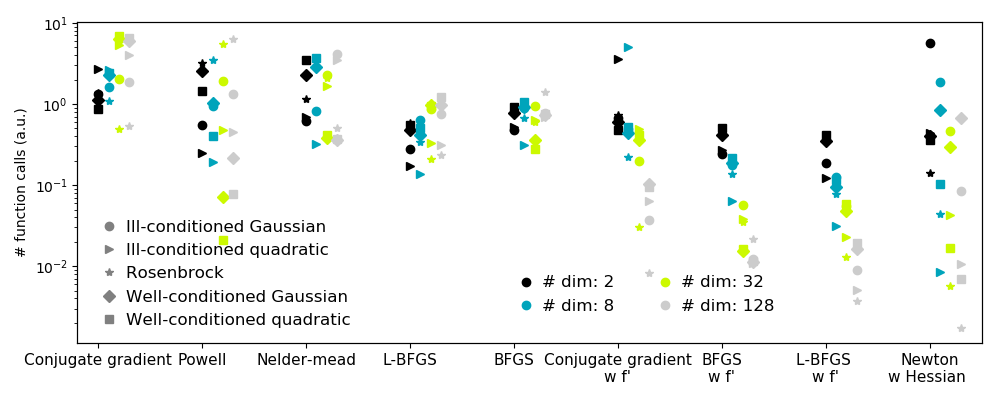
2.7.5.4. Synthetic exercices
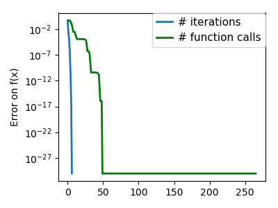
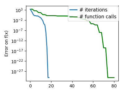
Exercice: A simple (?) quadratic function
Optimize the following function, using K[0] as a starting point:
np.random.seed(0)
K = np.random.normal(size=(100, 100))

def f(x):
    return np.sum((np.dot(K, x - 1))**2) + np.sum(x**2)**2
Time your approach. Find the fastest approach. Why is BFGS not
working well?
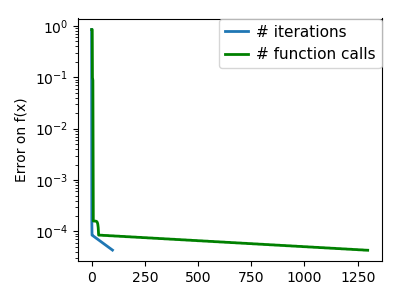
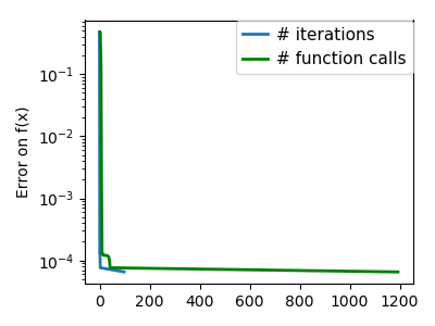
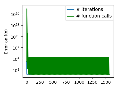
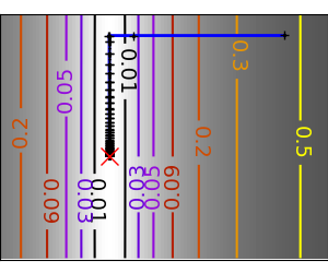
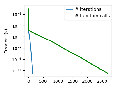
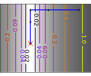
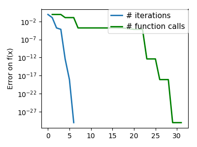
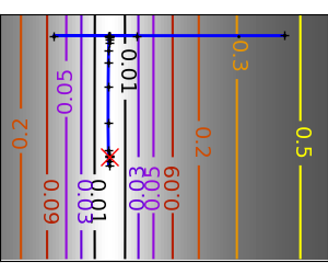
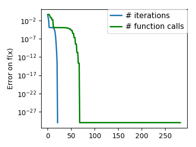
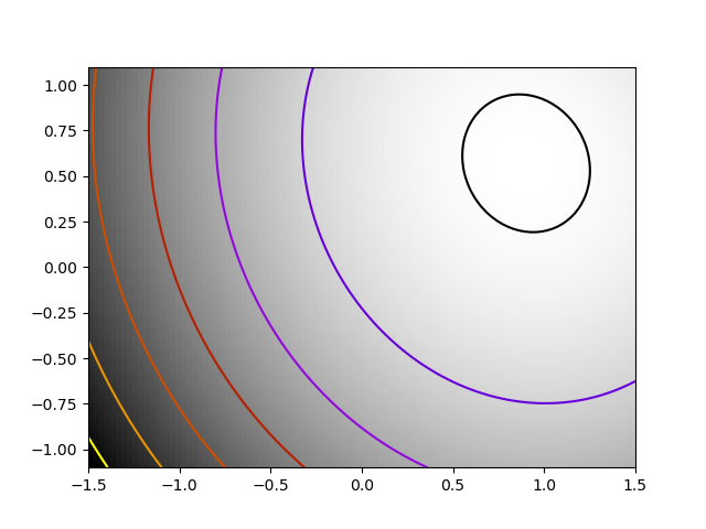
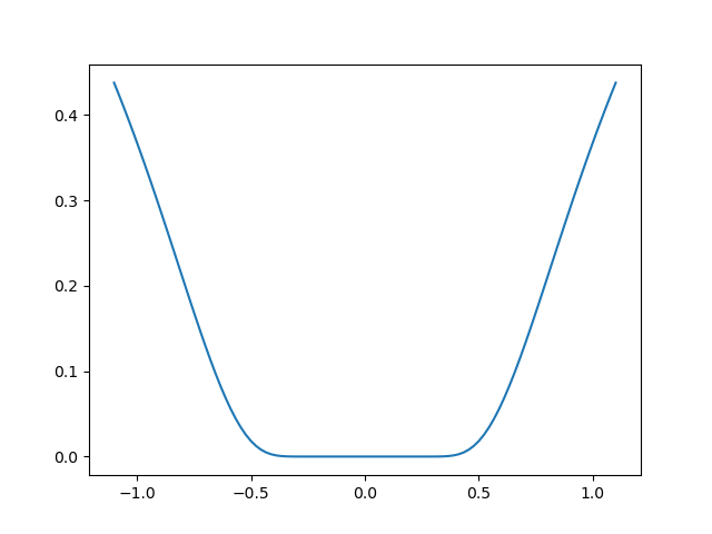
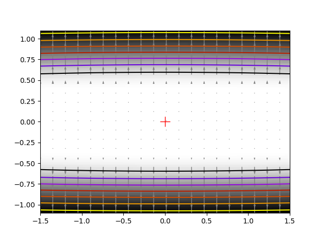
Exercice: A locally flat minimum
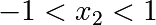
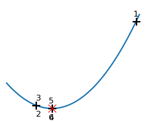
Consider the function exp(-1/(.1*x**2 + y**2). This function admits
a minimum in (0, 0). Starting from an initialization at (1, 1), try
to get within 1e-8 of this minimum point.
2.7.6. Special case: non-linear least-squares
2.7.6.1. Minimizing the norm of a vector function
Least square problems, minimizing the norm of a vector function, have a
specific structure that can be used in the Levenberg–Marquardt algorithm
implemented in scipy.optimize.leastsq().
Lets try to minimize the norm of the following vectorial function:
>>> def f(x):
...     return np.arctan(x) - np.arctan(np.linspace(0, 1, len(x)))

>>> x0 = np.zeros(10)
>>> optimize.leastsq(f, x0)
(array([0.        ,  0.11111111,  0.22222222,  0.33333333,  0.44444444,
        0.55555556,  0.66666667,  0.77777778,  0.88888889,  1.        ]), 2)
This took 67 function evaluations (check it with ‘full_output=1’). What
if we compute the norm ourselves and use a good generic optimizer
(BFGS):
>>> def g(x):
...     return np.sum(f(x)**2)
>>> optimize.minimize(g, x0, method="BFGS")
  fun: 2.6940...e-11
 hess_inv: array([[...
 ...
           ...]])
      jac: array([...
 ...
           ...])
  message: ...'Optimization terminated successfully.'
     nfev: 144
      nit: 11
     njev: 12
   status: 0
  success: True
        x: array([-7.3...e-09,   1.1111...e-01,   2.2222...e-01, 3.3333...e-01,
        4.4444...e-01,   5.5555...e-01, 6.6666...e-01,   7.7777...e-01,
        8.8889...e-01, 1.0000...e+00])
BFGS needs more function calls, and gives a less precise result.
Note
leastsq is interesting compared to BFGS only if the
dimensionality of the output vector is large, and larger than the number
of parameters to optimize.
Warning
If the function is linear, this is a linear-algebra problem, and
should be solved with scipy.linalg.lstsq().
2.7.6.2. Curve fitting
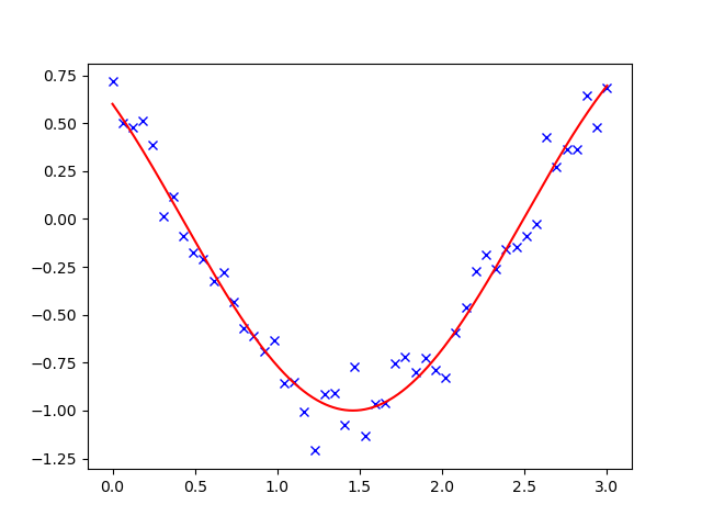
Least square problems occur often when fitting a non-linear to data.
While it is possible to construct our optimization problem ourselves,
scipy provides a helper function for this purpose:
scipy.optimize.curve_fit():
>>> def f(t, omega, phi):
...     return np.cos(omega * t + phi)

>>> x = np.linspace(0, 3, 50)
>>> y = f(x, 1.5, 1) + .1*np.random.normal(size=50)

>>> optimize.curve_fit(f, x, y)
(array([1.5185...,  0.92665...]), array([[ 0.00037..., -0.00056...],
       [-0.0005...,  0.00123...]]))
Exercise
Do the same with omega = 3. What is the difficulty?
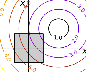
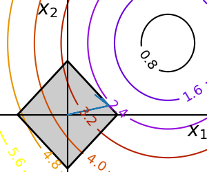
2.7.7. Optimization with constraints
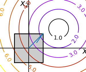
2.7.7.1. Box bounds
Box bounds correspond to limiting each of the individual parameters of
the optimization. Note that some problems that are not originally written
as box bounds can be rewritten as such via change of variables. Both
scipy.optimize.minimize_scalar() and scipy.optimize.minimize()
support bound constraints with the parameter bounds:
>>> def f(x):
...    return np.sqrt((x[0] - 3)**2 + (x[1] - 2)**2)
>>> optimize.minimize(f, np.array([0, 0]), bounds=((-1.5, 1.5), (-1.5, 1.5)))
      fun: 1.5811...
 hess_inv: <2x2 LbfgsInvHessProduct with dtype=float64>
      jac: array([-0.94868..., -0.31622...])
  message: ...'CONVERGENCE: NORM_OF_PROJECTED_GRADIENT_<=_PGTOL'
     nfev: 9
      nit: 2
   status: 0
  success: True
        x: array([1.5,  1.5])
2.7.7.2. General constraints
Equality and inequality constraints specified as functions: 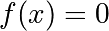
and  .
.
-
scipy.optimize.fmin_slsqp()Sequential least square programming:
equality and inequality constraints:
>>> def f(x):
...     return np.sqrt((x[0] - 3)**2 + (x[1] - 2)**2)

>>> def constraint(x):
...     return np.atleast_1d(1.5 - np.sum(np.abs(x)))

>>> x0 = np.array([0, 0])
>>> optimize.minimize(f, x0, constraints={"fun": constraint, "type": "ineq"})
     fun: 2.4748...
     jac: array([-0.70708..., -0.70712...])
 message: ...'Optimization terminated successfully.'
    nfev: 20
     nit: 5
    njev: 5
  status: 0
 success: True
       x: array([1.2500...,  0.2499...])
Warning
The above problem is known as the Lasso
problem in statistics, and there exist very efficient solvers for it
(for instance in scikit-learn). In
general do not use generic solvers when specific ones exist.
Lagrange multipliers
If you are ready to do a bit of math, many constrained optimization
problems can be converted to non-constrained optimization problems
using a mathematical trick known as Lagrange multipliers.
2.7.8. Full code examples
Updated: How do I find the minimum of a function on a closed interval [0,3.5] in Python? So far I found the max and min but am unsure how to filter out the minimum from here.
import sympy as sp

x = sp.symbols('x')

f = (x**3 / 3) - (2 * x**2) + (3 * x) + 1

fprime = f.diff(x)

all_solutions = [(xx, f.subs(x, xx)) for xx in sp.solve(fprime, x)]

print (all_solutions)
![]()
JohanC
70.1k8 gold badges32 silver badges64 bronze badges
asked Aug 28, 2016 at 15:05
![]()
2
Since this PR you should be able to do the following:
from sympy.calculus.util import *
f = (x**3 / 3) - (2 * x**2) - 3 * x + 1
ivl = Interval(0,3)
print(minimum(f, x, ivl))
print(maximum(f, x, ivl))
print(stationary_points(f, x, ivl))
answered Oct 25, 2019 at 19:55
![]()
smichrsmichr
16.2k2 gold badges23 silver badges33 bronze badges
2
Perhaps something like this
from sympy import solveset, symbols, Interval, Min
x = symbols('x')

lower_bound = 0
upper_bound = 3.5
function = (x**3/3) - (2*x**2) - 3*x + 1

zeros = solveset(function, x, domain=Interval(lower_bound, upper_bound))
assert zeros.is_FiniteSet # If there are infinite solutions the next line will hang.
ans = Min(function.subs(x, lower_bound), function.subs(x, upper_bound), *[function.subs(x, i) for i in zeros])
answered Aug 30, 2016 at 19:22
![]()
asmeurerasmeurer
85.6k26 gold badges167 silver badges240 bronze badges
2
Here’s a possible solution using sympy:
import sympy as sp

x = sp.Symbol('x', real=True)

f = (x**3 / 3) - (2 * x**2) - 3 * x + 1
#f = 3 * x**4 - 4 * x**3 - 12 * x**2 + 3

fprime = f.diff(x)

all_solutions = [(xx, f.subs(x, xx)) for xx in sp.solve(fprime, x)]
interval = [0, 3.5]
interval_solutions = filter(
    lambda x: x[0] >= interval[0] and x[0] <= interval[1], all_solutions)

print(all_solutions)
print(interval_solutions)
all_solutions is giving you all points where the first derivative is zero, interval_solutions is constraining those solutions to a closed interval. This should give you some good clues to find minimums and maximums 🙂
answered Aug 28, 2016 at 15:14
![]()
BPLBPL
10.4k8 gold badges57 silver badges115 bronze badges
4

The f.subs commands show two ways of displaying the value of the given function at x=3.5, the first as a rational approximation, the second as the exact fraction.

answered Aug 28, 2016 at 17:13
![]()
Bill BellBill Bell
20.9k5 gold badges42 silver badges58 bronze badges
