Как найти мощность гармоники

СИГНАЛОВ

7.1. Разложение периодических сигналов

по ортогональным функциям

Электрический сигнал
(токили напряжение)
называютпериодическим, если он
существует на интервале времени отдои удовлетворяет условию,
где– период сигнала, а– целое число. Примеры таких функций
времени показаны на рис. 7.1.

Рис. 7.1

При расчете разнообразных сигналов
удобно представить их взвешенной суммой
заданных функций времени вида

,
(7.1)

где
–
заданный набор (базис) функций
времени,– весовые коэффициенты, не зависящие от
времени. В этом случае функция времениможет описываться набором коэффициентов,от времени не зависящих.

Чтобы разложение в ряд (7.1) было взаимно
однозначным

144

функции
должны быть взаимноортогональнымина периоде сигнала, то есть должны
удовлетворять условию

(7.2)

где момент начала интегрирования
выбирается произвольно исходя из
удобства расчетов. Принабор функцийназываютортонормальным.

Для ортогонального базиса коэффициенты
разложения
определяются выражением

.
(7.3)

В математике и технике широко используются
различные ортогональные наборы функций
(базисы) и прежде всего гармонический
базис

,
(7.4)

полиномы Чебышева, Лагранжа, Эрмита и
др. В цифровой технике применяют
ортогональные дискретные функции Уолша,
Радамахера.

7.2. Ряд Фурье

Ряд Фурье для действительной периодической
функции времени
является ее разложением по ортогональному
базису (7.4) и имеет вид

145

(7.5)

Компоненту ряда Фурье вида

(7.6)

называют
-й
гармоникойсигнала,

(7.7)

– частота первой гармоники,–постоянная составляющая сигнала,

,
(7.8)

–амплитуда
-й
гармоникисигнала,

,
(7.9)

,
(7.10)

,
(7.11)

–начальная фаза
-й
гармоникисигнала,

146

(7.12)

Величины
иназываютамплитудами синфазной и
квадратурной составляющих-й
гармоники сигнала соответственно.

7.3. Спектры амплитуд и фаз периодического
сигнала

Периодический сигнал
взаимно однозначно описывается суммой
гармоник

,
(7.13)

то есть двумя в общем случае бесконечными
наборами чисел.

Первый из них называют спектром
амплитуд сигнала,

,
(7.14)

а второй – спектром фаз,

.
(7.15)

Спектры амплитуд и фаз не зависят от
времени, а определяются формой сигнала
на периоде колебаний. Частоты гармониккратны частоте первой гармоники,

,
(7.16)

147

не зависят от формы сигнала и определяются
только периодом его повторения
.

С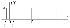пектры
сигнала можно представить в виде формулы,
таблицы или графика. В качестве примера
рассмотрим спектры амплитуд и фаз
последова-

Рис. 7.2 тельности
прямоугольных

импульсов
с амплитудой
,
длительностьюи периодом,
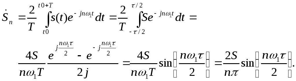
показанных на рис. 7.2. При расчетах
целесообразно выбрать момент начала
интегрирования.
Постоянная составляющая равна

,
(7.17)

а амплитуды синфазной и квадратурной
составляющих –

,
(7.18)

.
(7.19)

Для амплитуды и начальной фазы
-й
гармоники получим

,
(7.20)

(7.21)

148

Графики спектров амплитуд и фаз при
условии
,мс,мс
показаны на рис. 7.3а и рис. 7.3б соответственно.
Каждая гармоника отображается вертикальной
линией, длина которой равна величине
амплитуды или фазы.

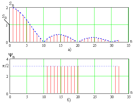
Рис. 7.3

Переменная
является номером гармоники. Ее можно
рассматривать как нормированную частоту
гармоники,

,

и спектральные диаграммы можно строить
в координатах частоты гармоники, как
показано на рис. 7.4 для спектра амплитуд.

Спектры имеют дискретный (линейчатый)
характер, интервал частот междусоседнимигармоникамиодинаков
и

149

равен
.

Спектр
амплитуд сверху всегда ограничен линией,
котораяпадает с ростом частоты(номера) гармоники. Вводится понятие
огибающей спектра амплитуд, определяемой
как непрерывная функция частоты,
которая в точкахточно совпадает со значениями

Рис. 7.4 амплитуд
гармоник. Формулу

огибающей
можно получить из выражения для спектра
амплитуд, подобного (7.20), при замене
номера гармоники
величиной

,
(7.22)

где
непрерывная переменная.

В примере (7.20) получим

,
(7.23)

график показан на рис. 7.3а пунктирной
линией. Характерной особенностью
огибающей спектра амплитуд сигнала
рис. 7.2 является наличие точек с нулевым
значением (нулей огибающей),
определяемых из уравнения

,
(7.24)

решение которого имеет вид

150

,
(7.25)

где
– целое число. Как видно, положение нулей
огибающей определяется только
длительностью импульса.

7.4. Синтез сигнала по его спектру

Если известны спектры амплитуд и фаз,
то с помощью ряда Фурье (7.13) можно получить
сигнал как функцию времени. Бесконечная
сумма на практике не реализуема и сигнал
описывается конечной суммой гармоник,

.
(7.26)

Соответствующие кривые при
,ипоказаны на рис. 7.5а, рис. 7.5б, и рис. 7.5в
соответственно.

Как видно, с увеличением
форма синтезированного сигнала
приближается к исходной (рис. 7.2).

7.5. Ряд Фурье в комплексной форме

Гармоники сигнала могут быть представлены
своими комплексными амплитудамив
виде

,
(7.27)

тогда исходный сигнал можно представить
в виде ряда Фурье,

.
(7.28)

151

Рис. 7.5

Амплитуда
-й
гармоникиравна модулю комплексной амплитуды,

,
(7.29)

а ее начальная фаза
– аргументус противоположным знаком,

152

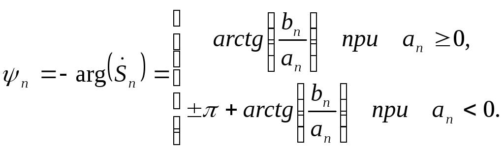
(7.30)

Комплексная амплитуда гармоники (2.27)
позволяет существенно упростить
расчеты спектров амплитуд и фазза
счет сокращения числа интегралов и с
учетом того, что подынтегральное
выражение с экспонентой часто интегрируется
проще, чем с тригонометрической функцией.

Рассмотрим сигнал, показанный на рис.
7.6, тогда

(7.31)

Как видно, в данном примере комплексная
амплитуда является действительнойвеличиной, что обусловлено формой
сигнала на рис. 7.2..Спектры амплитуд и
фаз совпадают с ранее полученными
значениями.

7.6. Влияние формы сигнала на спектры
амплитуд и фаз

Спектры амплитуд и фаз сигнала взаимно
однозначно связаны с его формой, которая
определяется формой импульсов и их
длительностью на периоде повторения.

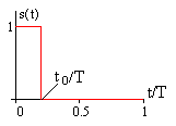
На рис. 7.6 показана последовательность
прямоугольных импульсов
длительностьюи с амплитудой 1 на интервале периодав нормированных координатах времени.
Для этого сигнала характерныкрутые
(с нулевой продолжи-

153

тельностью) фронт и срез импульса.
Величину

(7.32)

называют скважностьюимпульсов. На
рис. 7.7 приведены спектры амплитуд (рис.
7.7а) и фаз (рис. 7.7б)

Рис. 7.6 при
.

Рис. 7.7

На рис. 7.8 приведены аналогичные
зависимости при
.

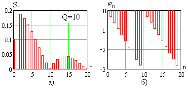
Рис. 7.8.

154

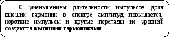
При фиксированном периоде повторения
импульсов
увеличение скважности означает уменьшение
длительности импульса,
при этом согласно рис. 7.7а и рис. 7.8а, а
также (7.20) амплитуды гармоник падают,
спектр амплитуд становится болееравномерным, положение нулей
огибающей спектра амплитуд смещается
в область более высоких частот (номеров
гармоник).

Рассмотрим трапециидальный импульс,
программа исследование которого в среде
MathCADпоказана на рис. 7.9.
Спектральный анализ проводится с помощью
стандартной процедуры спектрального
анализаfft(s).
Она построена на основе алгоритма
быстрого преобразования Фурье (БПФ)
и позволяет получить комплексные
коэффициенты,
с помощью которых комплексная амплитуда-й
гармоники определяется выражением

.
(7.33)

Период
сигнала выбран равным 1,–
число отсчетов сигнала на периоде.
Результаты расчета спектров амплитуд
и фаз приведены в листинге программы
на рис. 7.9 (повторите расчеты самостоятельно
для различных параметров сигнала).

Как видно при сравнении графиков спектров
амплитуд на рис. 7.7 и рис. 7.9, увеличение
длительности фронта и среза импульса
приводит к значительному ослаблению
высших гармоник сигнала.

155

На рис. 7.10 показан пример программы
расчета спектра амплитуд колоколообразного
сигнала вида

,
(7.34)

для которого характерно наиболее плавноеизменение значений во всем интервале
времени.

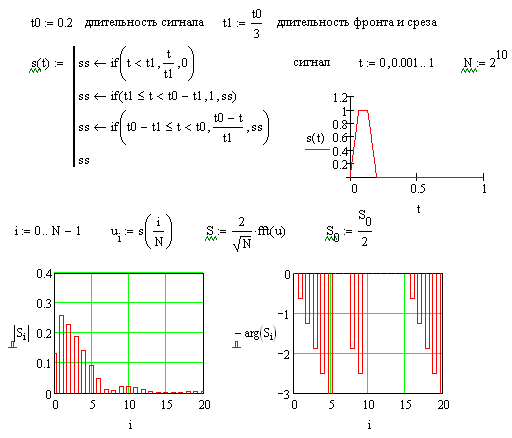
Рис. 7.9.

График сигнала и его спектр амплитуд
показаны в листинге программы на рис.
7.10. Как видно, спектр «гладкого» сигнала
сосредоточен в области нижних частот,
высшие гармоники практически отсутствуют.

Полученные выводы подтверждают результаты
синтеза прямоугольных импульсов по
ограниченному числу
гармоник, например, показанные на рис.
7.5.

156

Рис. 7.10.

7.7. Свойства спектров сигналов

Свойства спектров сигналов часто
формулируются в виде теорем.

Спектральное преобразование сигнала
линейно, то естькомплексная
амплитуда суммы сигналов равна сумме
комплексных амплитуд гармоник каждого
из суммируемых сигналов. На практике
особый интерес представляетсвойство
(теорема)смещения сигнала во
времени. Ее можно сформулировать
следующим образом.

157

Взяв модули левой и правой частей (7.30),
получим

,
(7.36)

то есть спектр амплитуд не изменяется
при задержке сиг-

нала во времени.

Вычислим аргументы обеих частей выражения
(7.30),

,
(7.37)

то есть начальные фазы гармоник сигнала
при временной задержке уменьшаются на
величину
,
которая зависит от номера гармоники,
периода сигнала (частоты его первой
гармоники) и величины задержки.

Для доказательства теоремы смещения
запишем

.
(7.38)

Проведем замену переменных
,
тогда получим

.
(7.39)

На спектральные характеристики влияют
свойства симметриисигнала.

Рассмотрим четныефункции времени,
удовлетворяющие условию.
В этом случае амплитуда квадратурной
составляющей-й
гармоники равна нулю

,
(7.40)

158

комплексная амплитуда
-й
гармоникиявляетсядействительнымчислом,

,
(7.41)

а начальная фаза равна 0 или
в зависимости от знака.

Для нечетнойфункции, удовлетворяющей
условию,
амплитуда синфазной составляющей-й
гармоники равна нулю

,
(7.42)

комплексная амплитуда
-й
гармоникиявляетсямнимым числом,

,
(7.43)

а начальная фаза равна 0 или
в зависимости от знака.

Эти свойства иллюстрирует пример четного
сигнала на рис. 7.2, для которого имеет
место равенство (7.19). Его фазовый спектр
со значениями 0 или
показан на рис. 7.3б.

Рассмотрим комплексные спектры двух
сигналов
(рис. 7.11а) и(рис. 7.11б), и их сумму(рис. 7.11в).

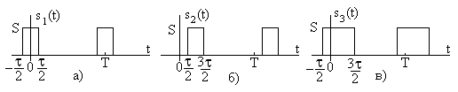
Рис. 7.11.

Сигнал
получен изсдвигом во времени на

159

величину
,
оба являются последовательностями
прямоугольных импульсов длительностью
импульса.
Сигналоказывается последовательностью
прямоугольных импульсов длительностью

Комплексная амплитуда
-й
гармоникиопределена ранее (7.31) и равна

(7.44)

По теореме смещенияможно найти
комплексную амплитуду-й
гармоники сигналав виде

.
(7.45)

Тогда согласно свойству линейностикомплексная амплитуда-й
гармоники сигналаравна

(7.46)

160

С другой стороны, при прямом вычислении
(проведите расчеты самостоятельно)
комплексная амплитуда-й
гармоники сигналаравна

,
(7.47)

что полностью совпадает с (7.46).

7.8. Мощность периодического сигнала

Пусть имеется сигнал
(ток или напряжение) в сопротивленииОм,
тогда средняя мощность сигнала равна

.
(7.48)

Эту же величину можно выразить через
гармоники сигнала с помощью равенства
(теоремы) Парсеваляв виде

.
(7.49)

С помощью спектральных характеристик
можно определить действующее значение
сигнала в виде

.
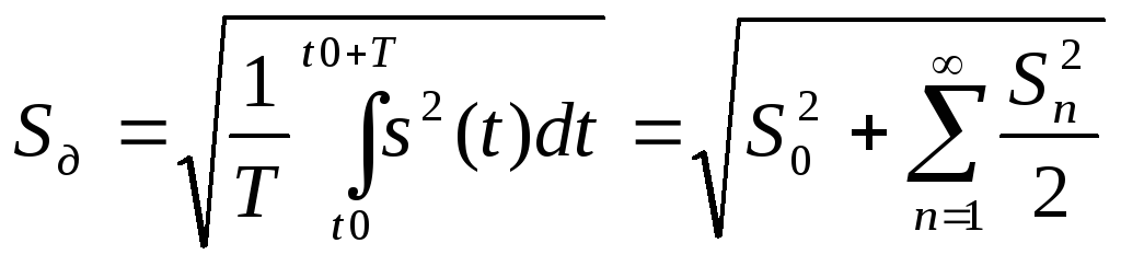(7.50)

7.9. Ширина спектра

Как видно по графикам спектров амплитуд
рассмотренных сигналов, в целом
наблюдается тенденция уменьшения

161

амплитуд гармоник с ростом их номера
(частоты). Графики на рис. 7.5 показывают,
что форма сигнала определяется
сравнительно небольшим числом гармоник.
Все это свидетельствует

о том, что для представления (даже
достаточно точного) сигнала необходимо
учитывать ограниченное число гармоник,
которые занимают конечный интервал
частот.

Мощность сигнала определяется выражением
(7.39). Для рассматриваемых видеосигналов
наиболее интенсивные гармоники имеют
номера от 1 до некоторой величины N,
при этом их суммарная мощность равна

.
(7.51)

Как видно, с ростом
мощностьувеличивается, и пристремится к полной мощности.

Тогда можно определить число гармоник
,
при котором мощностьбудет равна величине,
с помощью

выражения

.
(7.52)

В результате можно определить ширину
спектра
в виде

.
(7.53)

162

В качестве примера рассмотрим
последовательность прямоугольных
импульсов, показанную на рис. 7.2 со
спектром амплитуд, показанном на рис.
7.3а. (скважность импульсов
)
Зависимость нормированной мощностиот числа учитываемых гармоник показана
на рис. 7.12. Как видно, функцияявляетсянеубывающейи достигает
уровняпри(,),
тогда ширина спектра сигнала определяется
выражением (7.44).

Рис. 7.12

Этот же график в области значений от
0,9 до 1 показан на рис. 7.13. С ростом
кривая
очень медленно приближается к 1 и
достигает значения 0,99 уже при.

В инженерной практике рассмотренный
расчет ширины спектра проводится редко,
а используется ее инженерная оценка.Для импульсных сигналов с длительностью(на-

163

пример, рис. 7.2) ширина спектра определяется
выражением

(рад/с)
или(Гц)
(7.54)

(сравните эти величины со значениями
нулей огибающей спектра амплитуд).

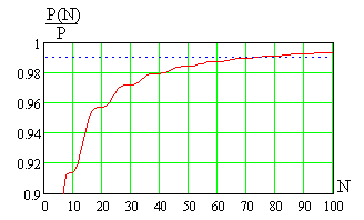
Рис. 7.13

Множитель от 1 до 3 косвенно характеризует
долю мощности сигнала, заключенную в
полосе пропускания (единица примерно
соответствует
,
а тройка – величине,
эти значения зависят от формы импульса).

Оценки ширины спектра можно выразить
через число гармоник,

,
(7.55)

где
требуемое число гармоник, равное

.
(7.56)

164

На практике чаще всего используются
соотношения с единичным множителем
вида

В рассмотренном примере сигнала на рис.
7.2 скважность
и для обеспечения 90% мощности необходимо
учитыватьгармоник (рис. 7.12), по оценке (7.58) требуется
учитывать 10 гармоник.

7.10. Задания для самостоятельного решения

Задание 7.1. Определите и постройте
графики спектров амплитуд и фаз сигналов
вида:

,

,

,

,

.

Задание 7.2. Определите спектры
амплитуд и фаз сигналов, показанных на
рис. 7.14, постройте их графики. Проведите
расчет ширины спектра при,и,
сравните полученные результаты.

165

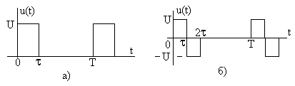
Рис. 7.14

Задание 7.3. С помощьютеоремы
смещенияпроведите расчет спектров
амплитуд и фаз сигнала, показанного на
рис. 7.14а, воспользовавшись результатами,
полученными для сигнала на рис.7.2.

Задание 7.4. Определите спектры
амплитуд и фаз сигнала, показанного на
рис.7.15, постройте их графики. Сравните
спектр амплитуд со спектром гармонического
сигнала, проанализируйте результаты.

Вычислите ширину спектра сигнала при
.
Чем обусловлены наблюдаемые различия
в ширине спектра для сигналов, показанных
на рис. 7.14а и рис. 7.15? Как в полученных
результатах проявляются свойства
симметрии сигнала?

Рис. 7.15

Задание 7.5. Определите спектры
амплитуд и фаз сигналjd,
показанного на рис.7.16, постройте их
графики.

166

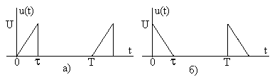
Рис. 7.16

Задание 7.6. Определите спектры
амплитуд и фаз сигнала, показанного на
рис.7.17, постройте их графики.

Рис. 7.17

Проведите тот же расчет, представив
сигнал на рис. 7.17 в виде суммы двух
импульсных последовательностей,
показанных на рис. 7.18, и используя
свойство линейности.

Рис. 7.18

167

In an electric power system, a harmonic of a voltage or current waveform is a sinusoidal wave whose frequency is an integer multiple of the fundamental frequency. Harmonic frequencies are produced by the action of non-linear loads such as rectifiers, discharge lighting, or saturated electric machines. They are a frequent cause of power quality problems and can result in increased equipment and conductor heating, misfiring in variable speed drives, and torque pulsations in motors and generators.

Harmonics are usually classified by two different criteria: the type of signal (voltage or current), and the order of the harmonic (even, odd, triplen, or non-triplen odd); in a three-phase system, they can be further classified according to their phase sequence (positive, negative, zero).

Current harmonics[edit]

In a normal alternating current power system, the current varies sinusoidally at a specific frequency, usually 50 or 60 hertz.
When a linear time-invariant electrical load is connected to the system, it draws a sinusoidal current at the same frequency as the voltage (though usually not in phase with the voltage).^[1]: 2

Current harmonics are caused by non-linear loads. When a non-linear load, such as a rectifier is connected to the system, it draws a current that is not necessarily sinusoidal. The current waveform distortion can be quite complex, depending on the type of load and its interaction with other components of the system. Regardless of how complex the current waveform becomes, the Fourier series transform makes it possible to deconstruct the complex waveform into a series of simple sinusoids, which start at the power system fundamental frequency and occur at integer multiples of the fundamental frequency.

In power systems, harmonics are defined as positive integer multiples of the fundamental frequency. Thus, the third harmonic is the third multiple of the fundamental frequency.

Harmonics in power systems are generated by non-linear loads. Semiconductor devices like transistors, IGBTs, MOSFETS, diodes etc are all non-linear loads. Further examples of non-linear loads include common office equipment such as computers and printers, fluorescent lighting, battery chargers and also variable-speed drives. Electric motors do not normally contribute significantly to harmonic generation. Both motors and transformers will however create harmonics when they are over-fluxed or saturated.

Non-linear load currents create distortion in the pure sinusoidal voltage waveform supplied by the utility, and this may result in resonance. The even harmonics do not normally exist in power system due to symmetry between the positive- and negative- halves of a cycle. Further, if the waveforms of the three phases are symmetrical, the harmonic multiples of three are suppressed by delta (Δ) connection of transformers and motors as described below.

If we focus for example on only the third harmonic, we can see how all harmonics with a multiple of three behaves in powers systems.^[2]

Power is supplied by a three phase system, where each phase is 120 degrees apart. This is done for two reasons: mainly because three-phase generators and motors are simpler to construct due to constant torque developed across the three phase phases; and secondly, if the three phases are balanced, they sum to zero, and the size of neutral conductors can be reduced or even omitted in some cases. Both these measures results in significant costs savings to utility companies. However, the balanced third harmonic current will not add to zero in the neutral. As seen in the figure, the 3rd harmonic will add constructively across the three phases. This leads to a current in the neutral wire at three times the fundamental frequency, which can cause problems if the system is not designed for it, (i.e. conductors sized only for normal operation.)^[2] To reduce the effect of the third order harmonics delta connections are used as attenuators, or third harmonic shorts as the current circulates in the delta the connection instead of flowing in the neutral of a Y-Δ transformer (wye connection).

Voltage harmonics[edit]

Voltage harmonics are mostly caused by current harmonics. The voltage provided by the voltage source will be distorted by current harmonics due to source impedance. If the source impedance of the voltage source is small, current harmonics will cause only small voltage harmonics. It is typically the case that voltage harmonics are indeed small compared to current harmonics. For that reason, the voltage waveform can usually be approximated by the fundamental frequency of voltage. If this approximation is used, current harmonics produce no effect on the real power transferred to the load. An intuitive way to see this comes from sketching the voltage wave at fundamental frequency and overlaying a current harmonic with no phase shift (in order to more easily observe the following phenomenon). What can be observed is that for every period of voltage, there is equal area above the horizontal axis and below the current harmonic wave as there is below the axis and above the current harmonic wave. This means that the average real power contributed by current harmonics is equal to zero. However, if higher harmonics of voltage are considered, then current harmonics do make a contribution to the real power transferred to the load.

A set of three line (or line-to-line) voltages in a balanced three-phase (three-wire or four-wire) power system cannot contain harmonics whose frequency is an integer multiple of the frequency of the third harmonics (i.e. harmonics of order ), which includes triplen harmonics (i.e. harmonics of order ).^[3] This occurs because otherwise Kirchhoff’s voltage law (KVL) would be violated: such harmonics are in phase, so their sum for the three phases is not zero, however KVL requires the sum of such voltages to be zero, which requires the sum of such harmonics to be also zero. With the same argument, a set of three line currents in a balanced three-wire three-phase power system cannot contain harmonics whose frequency is an integer multiple of the frequency of the third harmonics; but a four-wire system can, and the triplen harmonics of the line currents would constitute the neutral current.

Even, odd, triplen and non-triplen odd harmonics[edit]

The harmonics of a distorted (non-sinusoidal) periodic signal can be classified according to their order.

The cyclic frequency (in hertz) of the harmonics are usually written as or , and they are equal to or , where or is the order of the harmonics (which are integer numbers) and is the fundamental cyclic frequency of the distorted (non-sinusoidal) periodic signal. Similarly, the angular frequency (in radians per second) of the harmonics are written as or , and they are equal to or , where is the fundamental angular frequency of the distorted (non-sinusoidal) periodic signal. The angular frequency is related to the cyclic frequency as (valid for harmonics as well as the fundamental component).

Even harmonics[edit]

The even harmonics of a distorted (non-sinusoidal) periodic signal are harmonics whose frequency is a non-zero even integer multiple of the fundamental frequency of the distorted signal (which is the same as the frequency of the fundamental component). So, their order is given by:

where is an integer number; for example, . If the distorted signal is represented in the trigonometric form or the amplitude-phase form of the Fourier series, then takes only positive integer values (not including zero), that is it takes values from the set of natural numbers; if the distorted signal is represented in the complex exponential form of the Fourier series, then takes negative and positive integer values (not including zero, since the DC component is usually not considered as a harmonic).

Odd harmonics[edit]

The odd harmonics of a distorted (non-sinusoidal) periodic signal are harmonics whose frequency is an odd integer multiple of the fundamental frequency of the distorted signal (which is the same as the frequency of the fundamental component). So, their order is given by:

for example, .

In distorted periodic signals (or waveforms) that possess half-wave symmetry, which means the waveform during the negative half cycle is equal to the negative of the waveform during the positive half cycle, all of the even harmonics are zero () and the DC component is also zero (), so they only have odd harmonics (); these odd harmonics in general are cosine terms as well as sine terms, but in certain waveforms such as square waves the cosine terms are zero (, ). In many non-linear loads such as inverters, AC voltage controllers and cycloconverters, the output voltage(s) waveform(s) usually has half-wave symmetry and so it only contains odd harmonics.

The fundamental component is an odd harmonic, since when , the above formula yields , which is the order of the fundamental component. If the fundamental component is excluded from the odd harmonics, then the order of the remaining harmonics is given by:

for example, .

Triplen harmonics[edit]

The triplen harmonics of a distorted (non-sinusoidal) periodic signal are harmonics whose frequency is an odd integer multiple of the frequency of the third harmonic(s) of the distorted signal. So, their order is given by:

for example, .

All triplen harmonics are also odd harmonics, but not all odd harmonics are also triplen harmonics.

Non-triplen odd harmonics[edit]

Certain distorted (non-sinusoidal) periodic signals only possess harmonics that are not even harmonics nor triplen harmonics, for example the output voltage of a three-phase wye-connected AC voltage controller with phase angle control and a firing angle of and with a purely resistive load connected to its output and fed with three-phase sinusoidal balanced voltages. Their order is given by:

for example, .

All harmonics that are not even harmonics nor triplen harmonics are also odd harmonics, but not all odd harmonics are also harmonics that are not even harmonics nor triplen harmonics.

If the fundamental component is excluded from the harmonics that are not even nor triplen harmonics, then the order of the remaining harmonics is given by:

or also by:

for example, . In this latter case, these harmonics are called by IEEE as nontriple odd harmonics.^[4]

Positive sequence, negative sequence and zero sequence harmonics[edit]

In the case of balanced three-phase systems (three-wire or four-wire), the harmonics of a set of three distorted (non-sinusoidal) periodic signals can also be classified according to their phase sequence.^{[1]: 7–8 [5][3]}

Positive sequence harmonics[edit]

The positive sequence harmonics of a set of three-phase distorted (non-sinusoidal) periodic signals are harmonics that have the same phase sequence as that of the three original signals, and are phase-shifted in time by 120° between each other for a given frequency or order.^[6] It can be proven the positive sequence harmonics are harmonics whose order is given by:

for example, .^[5][3]

The fundamental components of the three signals are positive sequence harmonics, since when , the above formula yields , which is the order of the fundamental components. If the fundamental components are excluded from the positive sequence harmonics, then the order of the remaining harmonics is given by:^[1]

for example, .

Negative sequence harmonics[edit]

The negative sequence harmonics of a set of three-phase distorted (non-sinusoidal) periodic signals are harmonics that have an opposite phase sequence to that of the three original signals, and are phase-shifted in time by 120° for a given frequency or order.^[6] It can be proven the negative sequence harmonics are harmonics whose order is given by:^[1]

for example, .^[5][3]

Zero sequence harmonics[edit]

The zero sequence harmonics of a set of three-phase distorted (non-sinusoidal) periodic signals are harmonics that are in phase in time for a given frequency or order. It can be proven the zero sequence harmonics are harmonics whose frequency is an integer multiple of the frequency of the third harmonics.^[1] So, their order is given by:

for example, .^[5][3]

All triplen harmonics are also zero sequence harmonics,^[1] but not all zero sequence harmonics are also triplen harmonics.

Total harmonic distortion[edit]

Total harmonic distortion, or THD is a common measurement of the level of harmonic distortion present in power systems. THD can be related to either current harmonics or voltage harmonics, and it is defined as the ratio of the RMS value of all harmonics to the RMS value of the fundamental component times 100%; the DC component is neglected.

where V_k is the RMS voltage of the kth harmonic, I_k is the RMS current of the kth harmonic, and k = 1 is the order of the fundamental component.

It is usually the case that we neglect higher voltage harmonics; however, if we do not neglect them, real power transferred to the load is affected by harmonics. Average real power can be found by adding the product of voltage and current (and power factor, denoted by pf here) at each higher frequency to the product of voltage and current at the fundamental frequency, or

where V_k and I_k are the RMS voltage and current magnitudes at harmonic k ( denotes the fundamental frequency), and is the conventional definition of power without factoring in harmonic components.

The power factor mentioned above is the displacement power factor. There is another power factor that depends on THD. True power factor can be taken to mean the ratio between average real power and the magnitude of RMS voltage and current, .^[7]

and

Substituting this in for the equation for true power factor, it becomes clear that the quantity can be taken to have two components, one of which is the traditional power factor (neglecting the influence of harmonics) and one of which is the harmonics’ contribution to power factor:

Names are assigned to the two distinct factors as follows:

where is the displacement power factor and is the distortion power factor (i.e. the harmonics’ contribution to total power factor).

Effects[edit]

One of the major effects of power system harmonics is to increase the current in the system. This is particularly the case for the third harmonic, which causes a sharp increase in the zero sequence current, and therefore increases the current in the neutral conductor. This effect can require special consideration in the design of an electric system to serve non-linear loads.^[8]

In addition to the increased line current, different pieces of electrical equipment can suffer effects from harmonics on the power system.

Motors[edit]

Electric motors experience losses due to hysteresis and eddy currents set up in the iron core of the motor. These are proportional to the frequency of the current. Since the harmonics are at higher frequencies, they produce higher core losses in a motor than the power frequency would. This results in increased heating of the motor core, which (if excessive) can shorten the life of the motor. The 5th harmonic causes a CEMF (counter electromotive force) in large motors which acts in the opposite direction of rotation. The CEMF is not large enough to counteract the rotation; however it does play a small role in the resulting rotating speed of the motor.

Telephones[edit]

In the United States, common telephone lines are designed to transmit frequencies between 300 and 3400 Hz. Since electric power in the United States is distributed at 60 Hz, it normally does not interfere with telephone communications because its frequency is too low.

Sources[edit]

A pure sinusoidal voltage is a conceptual quantity produced by an ideal AC generator built with finely distributed stator and field windings that operate in a uniform magnetic field. Since neither the winding distribution nor the magnetic field are uniform in a working AC machine, voltage waveform distortions are created, and the voltage-time relationship deviates from the pure sine function. The distortion at the point of generation is very small (about 1% to 2%), but nonetheless it exists. Because this is a deviation from a pure sine wave, the deviation is in the form of a periodic function, and by definition, the voltage distortion contains harmonics.

When a sinusoidal voltage is applied to a linear time-invariant load, such as a heating element, the current through it is also sinusoidal. In non-linear and/or time-variant loads, such as an amplifier with a clipping distortion, the voltage swing of the applied sinusoid is limited and the pure tone is polluted with a plethora of harmonics.

When there is significant impedance in the path from the power source to a nonlinear load, these current distortions will also produce distortions in the voltage waveform at the load. However, in most cases where the power delivery system is functioning correctly under normal conditions, the voltage distortions will be quite small and can usually be ignored.

Waveform distortion can be mathematically analysed to show that it is equivalent to superimposing additional frequency components onto a pure sinewave. These frequencies are harmonics (integer multiples) of the fundamental frequency, and can sometimes propagate outwards from nonlinear loads, causing problems elsewhere on the power system.

The classic example of a non-linear load is a rectifier with a capacitor input filter, where the rectifier diode only allows current to pass to the load during the time that the applied voltage exceeds the voltage stored in the capacitor, which might be a relatively small portion of the incoming voltage cycle.

Other examples of nonlinear loads are battery chargers, electronic ballasts, variable frequency drives, and switching mode power supplies.

See also[edit]

• Power factor

Further reading[edit]

• Sankaran, C. (1999-10-01). “Effects of Harmonics on Power Systems”. Electrical Construction and Maintenance Magazine. Penton Media, Inc. Retrieved 2020-03-11.

References[edit]

Анонс: Общие принципы и сложности оценки потерь мощности в сетях с нелинейными нагрузками и гармоническими искажениями. Упрощенный расчет потерь активной энергии из-за присутствия в силовой сети высших гармоник.

Оценка потерь, связанных с гармониками, в распределительных сетях требует знания источников гармоник, характеристик элементов, участвующих в распространении гармонических токов, и, что наиболее важно и труднее всего оценить — периода, в течение которого гармонические токи присутствуют в системе. Профессиональный мониторинг сети (или ее сегмента) с определением спектра и амплитуд гармоник вплоть по 49 порядка дает неплохие результаты, но по факту данные для анализа сложно считать пригодными для расчетов, если не выполнен полный энергоаудит объекта с определением графика работы, режима в часы пиковой нагрузки и в период «отдыха» на выходные, праздники и т. д.

Некоторые энергосистемы имеют четко определенные периоды работы, например, использование люминесцентного освещения в коммерческих установках или работа электронного и цифрового оборудования в административных, складских помещениях в рабочее время. Однако промышленные предприятия представляют собой особый случай, поскольку здесь:

• имеют место различные автоматизированные процессы, многие из которых являются циклическими и часто сочетают в производственно-технологических процессах использование линейных и нелинейных нагрузок;
• работа энергетической системы, включая рабочее напряжение, конфигурации подстанций и служебных трансформаторов (типы подключения первичной и вторичной обмоток), а также их полное сопротивление утечки, регулирование напряжения и методы управления реактивной мощностью играют важную роль в оценке потерь;
• в силовых сетях большинства объектов практикуется использование схем подавления гармонических искажений, которые устраняют гармоники более высокого порядка, потому что эти потери связаны с квадратом тока;
• отмечается сложная определенность частот параллельных резонансов при включении и выключении конденсаторных батарей также остается ключевым моментом для оценки потерь, связанных с гармониками.

Упрощенный расчет потерь активной энергии из-за присутствия в силовой сети высших гармоник.

Повышенные среднеквадратичные значения тока из-за искажения гармонической формы волны приводят к повышенному тепловыделению в оборудовании и нежелательному срабатыванию предохранителей, а результирующий эффект может повлиять на жизненный цикл из-за ускоренного старения (деструкции) материалов изоляции трансформаторов, двигателей, диэлектрика конденсаторных батарей и т. д.

Обычно упрощенно рассматривают рассеивание тепла в электрических сетях как электрические потери величины I²R, а для случая гармонических искажений полные потери могут быть выражены зависимостью I²_RMS·Z, где I_RMS действующее (мгновенное, среднеквадратичное — Root Mean Square) значение тока, Z — сопротивление.

Если рассматривать только потери активной энергии и принять, что на активном (резистивном) сопротивлении амплитуды действующих токов гармоник прямо пропорциональны току на фундаментальной частоте и обратно пропорциональны их гармоническому порядку I_RMSⁿ=I_RMS^f·1/n, то для третьей гармоники I_RMS³=I_RMS^f·1/3=0.33·I_RMS^f, для пятой гармоники I_RMS⁵=I_RMS^f·1/5=0.2·I_RMS^f, для седьмой гармоники I_RMS⁷=I_RMS^f·1/7=0.14·I_RMS^f и т. д.

Если для примера принять, что через резистивный элемент цепи с сопротивлением 1 Ом протекает ток в 1 А, то без гармоник I_f = 1А, а активная мощность Р=1²·R=1 Вт при наличии 3-й, 5-й, 7-й гармоник в сети:

А общая активная мощность Р_общ=I_RMS²·R=1.08²·1=1.17 Вт. Тогда дополнительные потери активной мощности из-за гармоник составляют (Р_общ-Р)=1.17-1=0.17 или 17 %.

Если принять, что через то же сопротивление 1 Ом протекает ток 2 А, то без гармоник I_f=2А, а активная мощность Р=2²·R=4 Вт; при наличии 3-й, 5-й, 7-й гармоник в сети:

А общая активная мощность Р_общ=I_RMS²·R = 2.16²·1=4.67 Вт. Тогда дополнительные потери активной мощности из-за гармоник составляют (Р_общ-Р) = 4.67-4=0.67 или 67 %.

Важно
Несмотря на явное увеличение объема потерь активной энергии из-за гармоник при удваивании тока фундаментальной частоты общий коэффициент гармонических искажений

Т.е. по факту использование THD_I для оценки потерь оказывается мало информативным и не должно применяться для реальных расчетов.