Как найти плотность состояний - Сайт, где вы сможете решить свои вопросы

Текущая версия страницы пока не проверялась опытными участниками и может значительно отличаться от версии, проверенной 14 июня 2019 года; проверки требуют 9 правок.

Плотность состояний — величина, определяющая количество энергетических уровней в единичном интервале энергий на единицу объёма в трёхмерном случае (на единицу площади — в двумерном случае). Является важным параметром в статистической физике и физике твёрдого тела. Термин может применяться к фотонам, электронам, квазичастицам в твёрдом теле и т. п. Применяется только для одночастичных задач, то есть для систем, где можно пренебречь взаимодействием (невзаимодействующие частицы) или добавить взаимодействие в качестве возмущения (это приведёт к модификации плотности состояний).

Определение[править | править код]

Чтобы вычислить плотность состояний (число состояний в единичном энергетическом интервале) частицы, сначала найдём плотность состояний в обратном пространстве (импульсное или -пространство). «Расстояние» между состояниями определяется граничными условиями. Для свободных электронов и фотонов в области ${displaystyle 0<x<L_{x}}$ или для электронов в кристаллической решётке с размером решётки ${displaystyle L_{x}}$ используем периодические граничные условия Борна — фон Кармана для волновой функции: ${displaystyle psi (x)=psi (x+L_{x})}$ . С волновой функцией свободной частицы ${displaystyle psi (x)={mbox{const}}cdot e^{ikx}}$ получаем соотношения

${displaystyle 2pi N=kL_{x}qquad {frac {2pi }{L_{x}}}=Delta k}$

где — любое целое число, а — расстояние между состояниями с различными . Аналогичные соотношения имеют место и для других декартовых координат (, ).

Полное количество -состояний, доступных для частицы, — это объём -пространства, доступного для неё, делённый на объём -пространства, занимаемого одним состоянием. Доступный объём — это просто интеграл от до .

Объём -пространства для одного состояния в -мерном случае запишется в виде

$G(k)={frac {g_{s}}{left({Delta k}right)^{n}}}int limits _{0}^{k},{d^{n}{{mathbf {k}}}},$

где g_s — вырождение уровня (обычно это спиновое вырождение, равное 2). Это выражение нужно продифференцировать, чтобы найти плотность состояний в -пространстве: $g(k),dk={frac {dG(k)}{dk}},dk$ . Чтобы найти плотность состояний по энергии, нужно знать закон дисперсии для частицы, то есть выразить и в выражении в терминах и . Например для свободного электрона: $E={frac {p^{2}}{2m}}={frac {(hbar k)^{2}}{2m}}$ , $dE={frac {hbar ^{2}k}{m}},dk.$

С более общим определением связано соотношение

${displaystyle D(E)=sum _{s}~delta (E-E_{s})}$

(обычно подразумевают единичный объём, но при общей форме записи добавляется множитель ), где индекс соответствует некоторому состоянию дискретного или непрерывного спектра, а delta — дельта-функция. При переходе от суммирования к интегрированию по фазовому пространству размерности следует использовать правило

${displaystyle sum _{s}rightarrow int {frac {d^{n}p~d^{n}q}{(2pi hbar )^{n}}}}$

где hbar — постоянная Планка, — импульс, — пространственные координаты (в случае, если объём единичный, этот интеграл опускают).

Примеры[править | править код]

В таблице представлены выражения для плотности состояний электронов с параболическим законом дисперсии:

Доступный объём	Объём для одного состояния	Плотность состояний
${frac {4}{3}}pi k^{3}$	${frac {(2pi )^{3}}{L_{x}L_{y}L_{z}}}$	${frac {{sqrt {2m^{3}}}}{pi ^{2}hbar ^{3}}}{sqrt {E}}$
$pi k^{2}$	${frac {(2pi )^{2}}{L_{x}L_{y}}}$	${displaystyle {frac {m}{pi hbar ^{2}L_{z}}}sum _{l}Theta (E-E_{l})}$
	${frac {2pi }{L_{x}}}$	${displaystyle {frac {sqrt {2m}}{pi hbar L_{y}L_{z}}}sum _{l}{frac {1}{sqrt {E-E_{l}}}}}$
		${frac {2}{L_{x}L_{y}L_{z}}}sum _{l}delta (E-E_{l})$

где — индекс подзоны размерного квантования, Theta — функция Хевисайда. Формулы описывают случай, когда квантование по одному или нескольким направлениям связано с некоторым ограничивающим потенциалом.

Все формулы для , приведённые в самой правой колонке, имеют размерность Дж^-1м^-3 и структуру «некое выражение , делённое на произведение линейных размеров области квантования» — этих размеров столько, по скольким координатам ограничено движение. Если такое деление не производить (убрать все ), то останется с размерностью [ rho ] = Дж^-1м^-3, Дж^-1м^-2, Дж^-1м^-1 и Дж^-1, соответственно, для двумерного (2D), одномерного (1D) и нульмерного (0D) случаев. Под «плотностью состояний», в зависимости от контекста, может подразумеваться не только , но и .

Использование[править | править код]

Плотность состояний фигурирует в выражениях для расчёта концентрации частиц при их известном энергетическом распределении. Для фермионов, каковыми являются электроны, в условиях равновесия это распределение соответствует статистике Ферми — Дирака, а для бозонов, в том числе фотонов, — статистике Бозе — Эйнштейна.

Скажем, концентрации электронов (дырок) в зоне проводимости (валентной зоне) полупроводника в равновесии рассчитываются как

${displaystyle n=int limits _{E_{c}}^{+infty }rho (E)F(E),dE,quad p=int limits _{-infty }^{E_{v}}rho (E)(1-F(E)),dE}$

где — функция Ферми, ${displaystyle E_{c}}$ ( $E_{v}$ ) — энергия дна зоны проводимости (потолка валентной зоны). В качестве rho здесь должна быть подставлена формула для объекта соответствующей размерности: ${displaystyle rho _{3D}}$ для толщи материала (и тогда концентрации будут в м^-3), ${displaystyle rho _{2D}}$ для квантовой ямы (и тогда концентрацию получим в м^-2), ${displaystyle rho _{1D}}$ для квантовой проволоки (концентрацию получим в м^-1) или ${displaystyle rho _{0D}}$ (случай квантовой точки, получим не концентрацию, а число штук частиц).

Внешние ссылки[править | править код]

Britney Spears’ Guide to Semiconductor Physics Архивная копия от 14 мая 2011 на Wayback Machine

Источник

In solid state physics and condensed matter physics, the density of states (DOS) of a system describes the number of modes per unit frequency range. The density of states is defined as , where is the number of states in the system of volume whose energies lie in the range from to . It is mathematically represented as a distribution by a probability density function, and it is generally an average over the space and time domains of the various states occupied by the system. The density of states is directly related to the dispersion relations of the properties of the system. High DOS at a specific energy level means that many states are available for occupation.

Generally, the density of states of matter is continuous. In isolated systems however, such as atoms or molecules in the gas phase, the density distribution is discrete, like a spectral density. Local variations, most often due to distortions of the original system, are often referred to as local densities of states (LDOSs).

Introduction[edit]

In quantum mechanical systems, waves, or wave-like particles, can occupy modes or states with wavelengths and propagation directions dictated by the system. For example, in some systems, the interatomic spacing and the atomic charge of a material might allow only electrons of certain wavelengths to exist. In other systems, the crystalline structure of a material might allow waves to propagate in one direction, while suppressing wave propagation in another direction. Often, only specific states are permitted. Thus, it can happen that many states are available for occupation at a specific energy level, while no states are available at other energy levels .

Looking at the density of states of electrons at the band edge between the valence and conduction bands in a semiconductor, for an electron in the conduction band, an increase of the electron energy makes more states available for occupation. Alternatively, the density of states is discontinuous for an interval of energy, which means that no states are available for electrons to occupy within the band gap of the material. This condition also means that an electron at the conduction band edge must lose at least the band gap energy of the material in order to transition to another state in the valence band.

This determines if the material is an insulator or a metal in the dimension of the propagation. The result of the number of states in a band is also useful for predicting the conduction properties. For example, in a one dimensional crystalline structure an odd number of electrons per atom results in a half-filled top band; there are free electrons at the Fermi level resulting in a metal. On the other hand, an even number of electrons exactly fills a whole number of bands, leaving the rest empty. If then the Fermi level lies in an occupied band gap between the highest occupied state and the lowest empty state, the material will be an insulator or semiconductor.

Depending on the quantum mechanical system, the density of states can be calculated for electrons, photons, or phonons, and can be given as a function of either energy or the wave vector k. To convert between the DOS as a function of the energy and the DOS as a function of the wave vector, the system-specific energy dispersion relation between E and k must be known.

In general, the topological properties of the system such as the band structure, have a major impact on the properties of the density of states. The most well-known systems, like neutronium in neutron stars and free electron gases in metals (examples of degenerate matter and a Fermi gas), have a 3-dimensional Euclidean topology. Less familiar systems, like two-dimensional electron gases (2DEG) in graphite layers and the quantum Hall effect system in MOSFET type devices, have a 2-dimensional Euclidean topology. Even less familiar are carbon nanotubes, the quantum wire and Luttinger liquid with their 1-dimensional topologies. Systems with 1D and 2D topologies are likely to become more common, assuming developments in nanotechnology and materials science proceed.

Definition[edit]

The density of states related to volume V and N countable energy levels is defined as:

${displaystyle D(E)={frac {1}{V}},sum _{i=1}^{N}delta (E-E({mathbf {k} }_{i})).}$

Because the smallest allowed change of momentum for a particle in a box of dimension and length is ${displaystyle (Delta k)^{d}=({tfrac {2pi }{L}})^{d}}$ , the volume-related density of states for continuous energy levels is obtained in the limit as

${displaystyle D(E):=int _{mathbb {R} ^{d}}{frac {mathrm {d} ^{d}k}{(2pi )^{d}}}cdot delta (E-E(mathbf {k} )),}$

Here, is the spatial dimension of the considered system and the wave vector.

For isotropic one-dimensional systems with parabolic energy dispersion, the density of states is ${displaystyle D_{1D}(E)={tfrac {1}{2pi hbar }}({tfrac {2m}{E}})^{1/2}}$ . In two dimensions the density of states is a constant ${displaystyle D_{2D}={tfrac {m}{2pi hbar ^{2}}}}$ , while in three dimensions it becomes ${displaystyle D_{3D}(E)={tfrac {m}{2pi ^{2}hbar ^{3}}}(2mE)^{1/2}}$ .

Equivalently, the density of states can also be understood as the derivative of the microcanonical partition function ${displaystyle Z_{m}(E)}$ (that is, the total number of states with energy less than ) with respect to the energy:

${displaystyle D(E)={frac {1}{V}}cdot {frac {mathrm {d} Z_{m}(E)}{mathrm {d} E}}}$

The number of states with energy (degree of degeneracy) is given by:

${displaystyle gleft(E'right)=lim _{Delta Eto 0}int _{E'}^{E'+Delta E}D(E)mathrm {d} E=lim _{Delta Eto 0}Dleft(E'right)Delta E,}$

where the last equality only applies when the mean value theorem for integrals is valid.

Symmetry[edit]

There is a large variety of systems and types of states for which DOS calculations can be done.

Some condensed matter systems possess a structural symmetry on the microscopic scale which can be exploited to simplify calculation of their densities of states. In spherically symmetric systems, the integrals of functions are one-dimensional because all variables in the calculation depend only on the radial parameter of the dispersion relation. Fluids, glasses and amorphous solids are examples of a symmetric system whose dispersion relations have a rotational symmetry.

Measurements on powders or polycrystalline samples require evaluation and calculation functions and integrals over the whole domain, most often a Brillouin zone, of the dispersion relations of the system of interest. Sometimes the symmetry of the system is high, which causes the shape of the functions describing the dispersion relations of the system to appear many times over the whole domain of the dispersion relation. In such cases the effort to calculate the DOS can be reduced by a great amount when the calculation is limited to a reduced zone or fundamental domain.^[1] The Brillouin zone of the face-centered cubic lattice (FCC) in the figure on the right has the 48-fold symmetry of the point group O_h with full octahedral symmetry. This configuration means that the integration over the whole domain of the Brillouin zone can be reduced to a 48-th part of the whole Brillouin zone. As a crystal structure periodic table shows, there are many elements with a FCC crystal structure, like diamond, silicon and platinum and their Brillouin zones and dispersion relations have this 48-fold symmetry. Two other familiar crystal structures are the body-centered cubic lattice (BCC) and hexagonal closed packed structures (HCP) with cubic and hexagonal lattices, respectively. The BCC structure has the 24-fold pyritohedral symmetry of the point group T_h. The HCP structure has the 12-fold prismatic dihedral symmetry of the point group D_3h. A complete list of symmetry properties of a point group can be found in point group character tables.

In general it is easier to calculate a DOS when the symmetry of the system is higher and the number of topological dimensions of the dispersion relation is lower. The DOS of dispersion relations with rotational symmetry can often be calculated analytically. This result is fortunate, since many materials of practical interest, such as steel and silicon, have high symmetry.

In anisotropic condensed matter systems such as a single crystal of a compound, the density of states could be different in one crystallographic direction than in another. These causes the anisotropic density of states to be more difficult to visualize, and might require methods such as calculating the DOS for particular points or directions only, or calculating the projected density of states (PDOS) to a particular crystal orientation.

k-space topologies[edit]

Figure 1: Spherical surface in k-space for electrons in three dimensions.

The density of states is dependent upon the dimensional limits of the object itself. In a system described by three orthogonal parameters (3 Dimension), the units of DOS is Energy⁻¹Volume⁻¹ , in a two dimensional system, the units of DOS is Energy⁻¹Area⁻¹ , in a one dimensional system, the units of DOS is Energy⁻¹Length⁻¹. The referenced volume is the volume of k-space; the space enclosed by the constant energy surface of the system derived through a dispersion relation that relates E to k. An example of a 3-dimensional k-space is given in Fig. 1. It can be seen that the dimensionality of the system confines the momentum of particles inside the system.

Density of wave vector states (sphere)[edit]

The calculation for DOS starts by counting the N allowed states at a certain k that are contained within [k, k + dk] inside the volume of the system. This procedure is done by differentiating the whole k-space volume ${displaystyle Omega _{n,k}}$ in n-dimensions at an arbitrary k, with respect to k. The volume, area or length in 3, 2 or 1-dimensional spherical k-spaces are expressed by

$Omega _{n}(k)=c_{n}k^{n}$

for a n-dimensional k-space with the topologically determined constants

${displaystyle c_{1}=2, c_{2}=pi , c_{3}={frac {4pi }{3}}}$

for linear, disk and spherical symmetrical shaped functions in 1, 2 and 3-dimensional Euclidean k-spaces respectively.

According to this scheme, the density of wave vector states N is, through differentiating $Omega _{n,k}$ with respect to k, expressed by

${displaystyle N_{n}(k)={frac {{rm {d}}Omega _{n}(k)}{{rm {d}}k}}=n;c_{n};k^{n-1}}$

The 1, 2 and 3-dimensional density of wave vector states for a line, disk, or sphere are explicitly written as

${displaystyle {begin{aligned}N_{1}(k)&=2\N_{2}(k)&=2pi k\N_{3}(k)&=4pi k^{2}end{aligned}}}$

One state is large enough to contain particles having wavelength λ. The wavelength is related to k through the relationship.

$k={frac {2pi }{lambda }}$

In a quantum system the length of λ will depend on a characteristic spacing of the system L that is confining the particles. Finally the density of states N is multiplied by a factor $s/V_{k}$ , where s is a constant degeneracy factor that accounts for internal degrees of freedom due to such physical phenomena as spin or polarization. If no such phenomenon is present then s=1 . V_k is the volume in k-space whose wavevectors are smaller than the smallest possible wavevectors decided by the characteristic spacing of the system.

Density of energy states[edit]

To finish the calculation for DOS find the number of states per unit sample volume at an energy inside an interval . The general form of DOS of a system is given as

${displaystyle D_{n}left(Eright)={frac {{rm {d}}Omega _{n}(E)}{{rm {d}}E}}}$

The scheme sketched so far only applies to monotonically rising and spherically symmetric dispersion relations. In general the dispersion relation E(k) is not spherically symmetric and in many cases it isn’t continuously rising either. To express D as a function of E the inverse of the dispersion relation E(k) has to be substituted into the expression of $Omega _{n}(k)$ as a function of k to get the expression of $Omega _{n}(E)$ as a function of the energy. If the dispersion relation is not spherically symmetric or continuously rising and can’t be inverted easily then in most cases the DOS has to be calculated numerically. More detailed derivations are available.^[2]^[3]

Dispersion relations[edit]

The dispersion relation for electrons in a solid is given by the electronic band structure.

The kinetic energy of a particle depends on the magnitude and direction of the wave vector k, the properties of the particle and the environment in which the particle is moving. For example, the kinetic energy of an electron in a Fermi gas is given by

${displaystyle E=E_{0}+{frac {left(hbar kright)^{2}}{2m}} ,}$

where m is the electron mass. The dispersion relation is a spherically symmetric parabola and it is continuously rising so the DOS can be calculated easily.

Figure 2: Monatomic chain phonon dispersion relation

For longitudinal phonons in a string of atoms the dispersion relation of the kinetic energy in a 1-dimensional k-space, as shown in Figure 2, is given by

${displaystyle E=2hbar omega _{0}left|sin left({frac {ka}{2}}right)right|}$

where ${displaystyle omega _{0}={sqrt {k_{rm {F}}/m}}}$ is the oscillator frequency, the mass of the atoms, ${displaystyle k_{rm {F}}}$ the inter-atomic force constant and inter-atomic spacing. For small values of the dispersion relation is rather linear:

$E=hbar omega _{0}ka$

When the energy is

${displaystyle E=2hbar omega _{0}left|cos left({frac {pi -ka}{2}}right)right|}$

With the transformation and small this relation can be transformed to

${displaystyle E=2hbar omega _{0}left[1-left({frac {qa}{2}}right)^{2}right]}$

Isotropic dispersion relations[edit]

The two examples mentioned here can be expressed like

${displaystyle E=E_{0}+c_{k}k^{p}}$

This expression is a kind of dispersion relation because it interrelates two wave properties and it is isotropic because only the length and not the direction of the wave vector appears in the expression. The magnitude of the wave vector is related to the energy as:

${displaystyle k=left({frac {E-E_{0}}{c_{k}}}right)^{frac {1}{p}} ,}$

Accordingly, the volume of n-dimensional k-space containing wave vectors smaller than k is:

$Omega _{n}(k)=c_{n}k^{n}$

Substitution of the isotropic energy relation gives the volume of occupied states

${displaystyle Omega _{n}(E)={frac {c_{n}}{{c_{k}}^{frac {n}{p}}}}left(E-E_{0}right)^{frac {n}{p}} ,}$

Differentiating this volume with respect to the energy gives an expression for the DOS of the isotropic dispersion relation

${displaystyle D_{n}left(Eright)={frac {d}{dE}}Omega _{n}(E)={frac {nc_{n}}{p{c_{k}}^{frac {n}{p}}}}left(E-E_{0}right)^{{frac {n}{p}}-1}}$

Parabolic dispersion[edit]

Figure 3: Free-electron DOS in 3-dimensional k-space

In the case of a parabolic dispersion relation (p = 2), such as applies to free electrons in a Fermi gas, the resulting density of states, $D_{n}left(Eright)$ , for electrons in a n-dimensional systems is

${displaystyle {begin{aligned}D_{1}left(Eright)&={frac {1}{2{sqrt {c_{k}left(E-E_{0}right)}}}}\D_{2}left(Eright)&={frac {pi }{2c_{k}}}\D_{3}left(Eright)&=pi {sqrt {frac {E-E_{0}}{c_{k}^{3}}}} .end{aligned}}}$

for $E>E_{0}$ , with D(E)=0 for $E<E_{0}$ .

In 1-dimensional systems the DOS diverges at the bottom of the band as drops to $E_{0}$ . In 2-dimensional systems the DOS turns out to be independent of . Finally for 3-dimensional systems the DOS rises as the square root of the energy.^[4]

Including the prefactor $s/V_{k}$ , the expression for the 3D DOS is

${displaystyle N(E)={frac {V}{2pi ^{2}}}left({frac {2m}{hbar ^{2}}}right)^{frac {3}{2}}{sqrt {E-E_{0}}}}$

where is the total volume, and $N(E-E_{0})$ includes the 2-fold spin degeneracy.

Linear dispersion[edit]

In the case of a linear relation (p = 1), such as applies to photons, acoustic phonons, or to some special kinds of electronic bands in a solid, the DOS in 1, 2 and 3 dimensional systems is related to the energy as:

${displaystyle {begin{aligned}D_{1}left(Eright)&={frac {1}{c_{k}}}\D_{2}left(Eright)&={frac {2pi }{c_{k}^{2}}}left(E-E_{0}right)\D_{3}left(Eright)&={frac {4pi }{c_{k}^{3}}}left(E-E_{0}right)^{2}end{aligned}}}$

Distribution functions[edit]

The density of states plays an important role in the kinetic theory of solids. The product of the density of states and the probability distribution function is the number of occupied states per unit volume at a given energy for a system in thermal equilibrium. This value is widely used to investigate various physical properties of matter. The following are examples, using two common distribution functions, of how applying a distribution function to the density of states can give rise to physical properties.

Figure 4: The Fermi-Dirac probability distribution,

density of states, and

their product for a semiconductor. The lower green lobe depicts hole energy, and thus uses f(-x) as the distribution function.

Fermi–Dirac statistics: The Fermi–Dirac probability distribution function, Fig. 4, is used to find the probability that a fermion occupies a specific quantum state in a system at thermal equilibrium. Fermions are particles which obey the Pauli exclusion principle (e.g. electrons, protons, neutrons). The distribution function can be written as

${displaystyle f_{mathrm {FD} }(E)={frac {1}{exp left({frac {E-mu }{k_{mathrm {B} }T}}right)+1}}}$

is the chemical potential (also denoted as E_F and called the Fermi level when T=0), $k_{mathrm {B} }$ is the Boltzmann constant, and is temperature. Fig. 4 illustrates how the product of the Fermi-Dirac distribution function and the three-dimensional density of states for a semiconductor can give insight to physical properties such as carrier concentration and Energy band gaps.

Bose–Einstein statistics: The Bose–Einstein probability distribution function is used to find the probability that a boson occupies a specific quantum state in a system at thermal equilibrium. Bosons are particles which do not obey the Pauli exclusion principle (e.g. phonons and photons). The distribution function can be written as

${displaystyle f_{mathrm {BE} }(E)={frac {1}{exp left({frac {E-mu }{k_{rm {B}}T}}right)-1}}}$

From these two distributions it is possible to calculate properties such as the internal energy per unit volume , the number of particles , specific heat capacity , and thermal conductivity . The relationships between these properties and the product of the density of states and the probability distribution, denoting the density of states by g(E) instead of D(E) , are given by

${displaystyle {begin{aligned}u&=int E,f(E),g(E),{rm {d}}E\N&=Vint f(E),g(E),{rm {d}}E\c&={frac {partial }{partial T}}int E,f(E),g(E),{rm {d}}E\k&={frac {1}{d}}{frac {partial }{partial T}}int Ef(E),g(E),nu (E),Lambda (E),{rm {d}}Eend{aligned}}}$

is dimensionality, is sound velocity and Lambda is mean free path.

Applications[edit]

The density of states appears in many areas of physics, and helps to explain a number of quantum mechanical phenomena.

Quantization[edit]

Calculating the density of states for small structures shows that the distribution of electrons changes as dimensionality is reduced. For quantum wires, the DOS for certain energies actually becomes higher than the DOS for bulk semiconductors, and for quantum dots the electrons become quantized to certain energies.

Photonic crystals[edit]

The photon density of states can be manipulated by using periodic structures with length scales on the order of the wavelength of light. Some structures can completely inhibit the propagation of light of certain colors (energies), creating a photonic band gap: the DOS is zero for those photon energies. Other structures can inhibit the propagation of light only in certain directions to create mirrors, waveguides, and cavities. Such periodic structures are known as photonic crystals.^[5]^[6]^[7]^[8] In nanostructured media the concept of local density of states (LDOS) is often more relevant than that of DOS, as the DOS varies considerably from point to point.

Computational calculation[edit]

Interesting systems are in general complex, for instance compounds, biomolecules, polymers, etc. Because of the complexity of these systems the analytical calculation of the density of states is in most of the cases impossible. Computer simulations offer a set of algorithms to evaluate the density of states with a high accuracy. One of these algorithms is called the Wang and Landau algorithm.^[9]

Within the Wang and Landau scheme any previous knowledge of the density of states is required. One proceeds as follows: the cost function (for example the energy) of the system is discretized. Each time the bin i is reached one updates
a histogram for the density of states, g(i) , by

where f is called the modification factor. As soon as each bin in the histogram is visited a certain number of times
(10-15), the modification factor is reduced by some criterion, for instance,

${displaystyle f_{n+1}rightarrow {frac {1}{2}}f_{n}}$

where n denotes the n-th update step. The simulation finishes when the modification factor is less than a certain threshold, for instance ${displaystyle f_{n}<10^{-8}}$ .

The Wang and Landau algorithm has some advantages over other common algorithms such as multicanonical simulations and parallel tempering. For example, the density of states is obtained as the main product of the simulation. Additionally, Wang and Landau simulations are completely independent of the temperature. This feature allows to compute the density of states of systems with very rough energy landscape such as proteins.^[10]

Mathematically the density of states is formulated in terms of a tower of covering maps.^[11]

Local density of states[edit]

An important feature of the definition of the DOS is that it can be extended to any system. One of its properties are the translationally invariability which means that the density of the states is homogeneous and it’s the same at each point of the system. But this is just a particular case and the LDOS gives a wider description with a heterogeneous density of states through the system.

Concept[edit]

Local density of states (LDOS) describes a space-resolved density of states. In materials science, for example, this term is useful when interpreting the data from a scanning tunneling microscope (STM), since this method is capable of imaging electron densities of states with atomic resolution. According to crystal structure, this quantity can be predicted by computational methods, as for example with density functional theory.

A general definition[edit]

In a local density of states the contribution of each state is weighted by the density of its wave function at the point. becomes

${displaystyle n(E,x)=sum _{j}|phi _{j}(x)|^{2}delta (E-varepsilon _{j})}$

the factor of ${displaystyle |phi _{j}(x)|^{2}}$ means that each state contributes more in the regions where the density is high. An average over of this expression will restore the usual formula for a DOS. The LDOS is useful in inhomogeneous systems, where contains more information than alone.

For a one-dimensional system with a wall, the sine waves give

${displaystyle n_{1D}(E,x)={frac {2}{pi hbar }}{sqrt {frac {2m}{E}}}sin ^{2}{kx}}$

where .

In a three-dimensional system with x>0 the expression is

${displaystyle n_{3D}(E,x)=left(1-{frac {sin {2kx}}{2kx}}right)n_{3D}(E)}$

In fact, we can generalise the local density of states further to

${displaystyle n(E,x,x')=sum _{j}phi _{j}(x)phi _{j}^{*}(x')delta (E-varepsilon _{j})}$

this is called the spectral function and it’s a function with each wave function separately in its own variable. In more advanced theory it is connected with the Green’s functions and provides a compact representation of some results such as optical absorption.

Space resolved local density of states. A sequence of images with varying gate bias in a nanowire MOSFET at drain bias Vd=0.6V. Notice the confined energy levels as they move with increasing gate bias.

Solid state devices[edit]

LDOS can be used to gain profit into a solid-state device. For example, the figure on the right illustrates LDOS of a transistor as it turns on and off in a ballistic simulation. The LDOS has clear boundary in the source and drain, that corresponds to the location of band edge. In the channel, the DOS is increasing as gate voltage increase and potential barrier goes down.

Optics and photonics[edit]

In optics and photonics, the concept of local density of states refers to the states that can be occupied by a photon. For light it is usually measured by fluorescence methods, near-field scanning methods or by cathodoluminescence techniques. For different photonic structures, the LDOS have different behaviors and they are controlling spontaneous emission in different ways. In photonic crystals, the near-zero LDOS are expected and they cause inhibition in the spontaneous emission.^[12]
The LDOS are still in photonic crystals but now they are in the cavity. In this case, the LDOS can be much more enhanced and they are proportional with Purcell enhancements of the spontaneous emission.^[13]^[14]
Similar LDOS enhancement is also expected in plasmonic cavity.^[15]
However, in disordered photonic nanostructures, the LDOS behave differently. They fluctuate spatially with their statistics are proportional to the scattering strength of the structures.^[16]
In addition, the relationship with the mean free path of the scattering is trivial as the LDOS can be still strongly influenced by the short details of strong disorders in the form of a strong Purcell enhancement of the emission.^[17]
and finally, for the plasmonic disorder, this effect is much stronger for LDOS fluctuations as it can be observed as a strong near-field localization.^[18]

References[edit]

^
Walter Ashley Harrison (1989). Electronic Structure and the Properties of Solids. Dover Publications. ISBN 978-0-486-66021-9.
^ Sample density of states calculation
^ Another density of states calculation
^ Charles Kittel (1996). Introduction to Solid State Physics (7th ed.). Wiley. Equation (37), p. 216. ISBN 978-0-471-11181-8.
^
Yablonovitch, E. (1987). “Inhibited Spontaneous Emission in Solid-State Physics and Electronics”. Phys. Rev. Lett. 58 (20): 2059–2062. Bibcode:1987PhRvL..58.2059Y. doi:10.1103/PhysRevLett.58.2059. PMID 10034639.
^
John, Sajeev; Wang, Jian (1990). “Quantum electrodynamics near a photonic band gap: Photon bound states and dressed atom”. Phys. Rev. Lett. 64 (20): 2418–2421. Bibcode:1990PhRvL..64.2418J. doi:10.1103/PhysRevLett.64.2418. PMID 10041707.
^
Lodahl, P.; van Driel, A. F.; Nikolaev, I. (2004). “Controlling the dynamics of spontaneous emission from quantum dots by photonic crystals”. Nature. 430 (1): 654–657. Bibcode:2004Natur.430..654L. doi:10.1038/nature02772. hdl:1874/16698. PMID 15295594. S2CID 4334567.
^
Fujita, Masayuki; Takahashi, Shigeki; Tanaka, Yoshinori; Asano, Takashi; Noda, Susumu (2005). “Simultaneous Inhibition and Redistribution of Spontaneous Light Emission in Photonic Crystals”. Science. 308 (5726): 1296–1298. Bibcode:2005Sci…308.1296F. doi:10.1126/science.1110417. PMID 15919989. S2CID 30116866.
^
Wang, Fugao; Landau, D. P. (2001). “Efficient, Multiple-Range Random Walk Algorithm to Calculate the Density of States”. Phys. Rev. Lett. 86 (10): 2050–2053. arXiv:cond-mat/0011174. Bibcode:2001PhRvL..86.2050W. doi:10.1103/PhysRevLett.86.2050. PMID 11289852. S2CID 2941153.
^ Ojeda, P.; Garcia, M. (2010). “Electric Field-Driven Disruption of a Native beta-Sheet Protein Conformation and Generation of a Helix-Structure”. Biophysical Journal. 99 (2): 595–599. Bibcode:2010BpJ….99..595O. doi:10.1016/j.bpj.2010.04.040. PMC 2905109. PMID 20643079.
^
Adachi T. and Sunada. T (1993). “Density of states in spectral geometry of states in spectral geometry”. Comment. Math. Helvetici. 68: 480–493. doi:10.1007/BF02565831. S2CID 120828817.
^
Sprik, R.; van Tiggelen, B. A.; Lagendijk, A. (1996). “Density of states in spectral geometry of states in spectral geometry”. Europhys. Lett. 35 (4): 265–270. doi:10.1209/epl/i1996-00564-y. S2CID 250854036.
^
Englund, Dirk; Fattal, David; Waks, Edo; Solomon, Glenn; Zhang, Bingyang; Nakaoka, Toshihiro; Arakawa, Yasuhiko; Yamamoto, Yoshihisa; Vuckovic, Jelena (2005). “Controlling the Spontaneous Emission Rate of Single Quantum Dots in a Two-Dimensional Photonic Crystal”. Phys. Rev. Lett. 95 (1): 013904. arXiv:quant-ph/0501091. Bibcode:2005PhRvL..95a3904E. doi:10.1103/PhysRevLett.95.013904. PMID 16090618. S2CID 9049385.
^
Birowosuto, M.; Sumikura, H.; Matsuo, S.; Notomi, M. (2012). “Fast Purcell-enhanced single photon source in 1,550-nm telecom band from a resonant quantum dot-cavity coupling”. Sci. Rep. 2 (1): 321. arXiv:1203.6171. Bibcode:2012NatSR…2E.321B. doi:10.1038/srep00321. PMC 3307054. PMID 22432053.
^
Farahani, J. N.; Pohl, D. W.; Eisler, H.-J.; Hecht, B. (2005). “Single Quantum Dot Coupled to a Scanning Optical Antenna: A Tunable Superemitter”. Phys. Rev. Lett. 95 (1): 017402. Bibcode:2005PhRvL..95a7402F. doi:10.1103/PhysRevLett.95.017402. PMID 16090656.
^
Birowosuto, M.; Skipetrov, S.; Vos, W.; Mosk, A. (2010). “Observation of Spatial Fluctuations of the Local Density of States in Random Photonic Media”. Phys. Rev. Lett. 105 (1): 013904. arXiv:1002.3186. Bibcode:2010PhRvL.105a3904B. doi:10.1103/PhysRevLett.105.013904. PMID 20867448. S2CID 25044558.
^
Sapienza, R.; Bondareff, P.; Pierrat, R.; Habert, B.; Carminati, R.; van Hulst, N. F. (2011). “Long-Tail Statistics of the Purcell Factor in Disordered Media Driven by Near-Field Interactions”. Phys. Rev. Lett. 106 (16): 163902. Bibcode:2011PhRvL.106p3902S. doi:10.1103/PhysRevLett.106.163902. PMID 21599367.
^
Krachmalnicoff, V.; Castanié, E.; De Wilde, Y.; Carminati, R. (2010). “Long-Tail Statistics of the Purcell Factor in Disordered Media Driven by Near-Field Interactions”. Phys. Rev. Lett. 105 (18): 183901. arXiv:1007.3691. doi:10.1103/PhysRevLett.105.183901. PMID 21231105. S2CID 15590513.

External links[edit]

Online lecture:ECE 606 Lecture 8: Density of States by M. Alam
Scientists shed light on glowing materials How to measure the Photonic LDOS

Источник

Все основные свойства электронных нитей
определяются их законом дисперсии, т.
е. зависимостью энергии от импульса,
определяемой формулой (4.1). В этой связи
очень интересно сравнить между собой
электронные системы различных
размерностей: массивные полупроводники
с законом дисперсии Е =(р²_х
+ р²_y
+ р²_z)/2т,
двумерные структуры с законом дисперсииЕ= E_N
+ (p²_x
+ р²_у)/2т и
квантовые нити. Несмотря на внешнее
сходство приведенных формул, разное
число направлений, по которым электроны
могут свободно двигаться, вызовет
качественное различие почти во всех
свойствах.

Важнейшей характеристикой электронной
системы наряду с ее законом дисперсии
является плотность состояний, т. е. число
состояний в единичном интервале энергии.
Поскольку электроны подчиняются принципу
Паули, то плотность состояний определит
то максимальное число электронов,
которое может разместиться в данном
интервале энергий, а уж распределение
электронов по энергиям определит все
их остальные свойства.

Основной вопрос здесь заключается в
следующем: насколько должны отличаться
импульсы двух электронов, чтобы они
могли считаться принадлежащими к
различным квантовым состояниям и не
подчиняться принципу Паули? Пусть размер
образца вдоль оси х равенL_x.
Из соотношений неопределенности
квантовой механики следует, что при
этом неопределенность импульсар_х
будет равна2πћ/L_xи, следовательно, различными могут
считаться состояния со значениями
импульса, различающимися на2πћ/L.Аналогичные рассуждения относятся
и к другим направлениям, в которых
электроны двигаются как свободные.

Теперь можно вычислить важную промежуточную
характеристику системы G(E)
– полное число состояний, имеющих
энергию, меньшую, чемЕ. В трехмерном
случае:

,
(4.2)

где V
– объем образца,aV_p
– объем так называемого импульсногопространства, т. е.
области в осях р_х,
р_у,
p_z,
,для которой
энергия электрона (р_х
²+
p_y²
+ р_z²)/2т
меньше,
чемЕ. Легко понять, что эта область
представляет собой шар радиусомc:j2mE
и объемом(4π/3)(2тЕ)^3/2,
так что окончательно в трехмерном
случае.

Очевидно, что G(E)
образовалось
суммированием всех состояний с
энергиями от 0 доЕ. При этом
интересующая нас плотность состояний
вблизи заданной энергии будет определяться
производнойG по
энергии. Кроме того, обычно интересуютсяплотностью состояний
в расчете не на весь образец, а
на единицу объема и учитывают то, что в
каждом состоянии
могут находиться два электрона с
противоположными спинами. Это дает
окончательную формулу для трехмерной
плотности состояний:

.
(4.3)

В двумерном случае для каждого из
квантово-размерных уровней с энергией
E_Nполное число состоянийG_N(E)=
m(E
– E_N)S/(2πћ²),
S – площадь
образца. Плотность состояний, которая
в этом случае вычисляется на единицу
площади, определяется суммой по всем
уровням, энергии которыхE_N
лежат нижеЕ:

.
(4.4)

Наконец, для каждого
уровня Е_i
квантовой
нити длинойL и
плотность состояний на единицу длины

(4.5)

На рис. 4.2 схематично показаны функции
плотности состояний для всех обсуждавшихся
случаев. Видно, что они носят качественно
различный характер.


	Рис. 4.2. Плотность состояний в массивном трехмерном полупроводнике (а), в двумерных электронных структурах – квантовых ямах (б) и одномерных структурах – квантовых нитях (в)

В трехмерном случае плотность состояний
монотонно растет с энергией, в двумерном
случае имеет вид горизонтальных ступенек,
а в квантовых нитях неограниченно растет
каждый раз, если необходимо сделать
оценку величины энергии очередного
квантового уровня.

Соседние файлы в папке ФПЦП

Источник

Основы квантовых вычислений: чистые и смешанные состояния

Время на прочтение
4 мин

Количество просмотров 15K

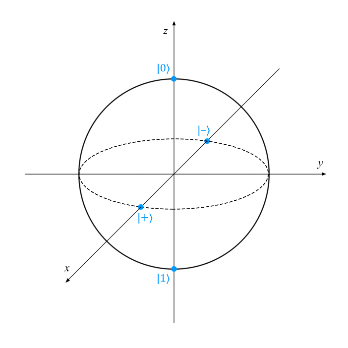
Недавно мы рассказали о способе наглядного представления однокубитных состояний — сфере Блоха. Всем чистым состояниям соответствуют точки на поверхности сферы Блоха, а смешанным — точки внутри нее. В этой публикации мы постараемся объяснить, что на самом деле представляют собой чистые и смешанные состояния.

Статьи из цикла:

Квантовые вычисления и язык Q# для начинающих

Введение в квантовые вычисления

Квантовые цепи и вентили — вводный курс

Основы квантовых вычислений: чистые и смешанные состояния

Квантовая телепортация на языке Q#

Квантовые вычисления: справочные материалы

Строгое математическое объяснение приводится в книге М. Нильсена И. Чанг «Квантовая информация и квантовые вычисления», в разделе 2.4.1: «Ансамбли квантовых состояний», а также в этих замечательных конспектах (и в соответствующих записях лекций) профессора Леонарда Зюскинда из Стендфордского университета.

Чистые состояния

Чистым называется состояние, которое можно представить одним вектором состояния |ψι〉. С практической точки зрения это означает, что в любой момент времени мы точно (с вероятностью 100 %) знаем, что наша система находится в состоянии |ψι〉. Другими словами, если система находится в чистом состоянии, мы обладаем полным представлением о ней и точно знаем, в каком состоянии она находится.

Примеры чистых состояний: |0〉, |1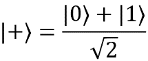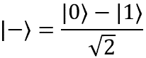〉, , . Им соответствуют следующие точки на поверхности сферы Блоха:

Смешанные состояния

Если полного представления о том, в каком состоянии находится подготовленная система, нет, то говорят, что она находится в смешанном состоянии. Такая ситуация может быть вызвана множеством причин: например, некорректной настройкой лабораторного оборудования или спутанностью частиц с внешней системой, которая нам недоступна. Как бы то ни было, если система находится в смешанном состоянии, мы не можем быть на 100 % уверены, находится ли она в чистом состоянии или либо в любом другом возможном состоянии. В таком случае состояние системы описывается вероятностным распределением всех чистых состояний, в которых она с ненулевой вероятностью может находиться после подготовки.

Рассмотрим пример. Допустим, наша коллега Мэри подготовила кубиты для нашего эксперимента. Она пытается саботировать работу и не говорит нам, в каком состоянии находится каждый кубит, но мы знаем, что возможных вариантов всего три: это чистые состояния . Поэтому наше стартовое состояние необходимо описать на языке теории вероятностей: . Такое сочетание чистых состояний называют смешанным состоянием.

Пусть мы знаем, что Мэри (например) подготавливает состояние в два раза чаще, чем или . Мы можем использовать это знание, чтобы описать вероятности возможных состояний нашей системы к началу эксперимента. Если мы не знаем, как именно Мэри выбирает подготавливаемые состояния, то следует предположить, что все они равновероятны. И сейчас пришло время рассказать о матрице плотности (или операторе плотности).

Оператор плотности, ρ

Оператор плотности (ρ) можно использовать для представления состояния системы, начальное состояние которой не известно наверняка. Этот оператор является обобщением векторов состояния (которые используется для записи чистых состояний). Матрица плотности для чистого состояния естественным образом вырождается в вектор состояния |ψι〉. Для тех, кому это интересно, ниже приводятся некоторые математические выкладки.

Немного математики

ПРИМЕЧАНИЕ. Предполагается, что читатель владеет базовыми понятиями векторной и матричной алгебры: внешнее и внутреннее произведение, ортогональность и т. п. Для знакомства с ними рекомендуется обратиться к книге М. Нильсена и И. Чанг или к Стендфордским лекциям, которые упомянуты в начале статьи.
Оператор плотности можно определить как

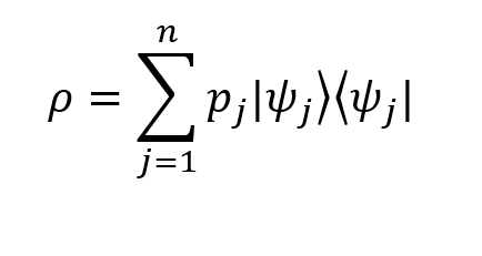
Здесь:

В нашем примере оператор плотности раскрывается следующим образом:

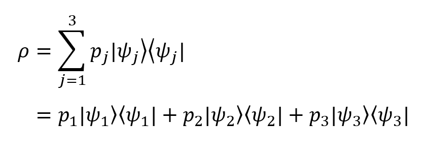
Если подставить значения вероятности из рассмотренного выше примера, получим

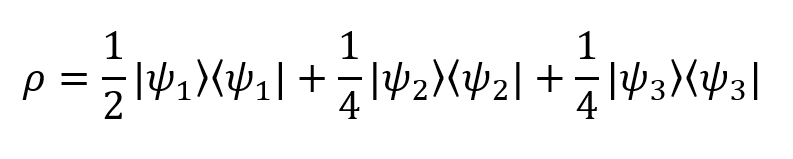
Это и есть матрица плотности нашей воображаемой системы! Не так уж сложно.
После того как мы вычислили оператор плотности, найти вероятность того, что измерение ρ покажет некоторое чистое квантовое состояние |ψ〉, очень просто: она равна 〈ψ|ρ|ψ〉.

В том случае, если состояние является чистым (то есть изначально система может находиться только в одном состоянии), выполняется следующее равенство:

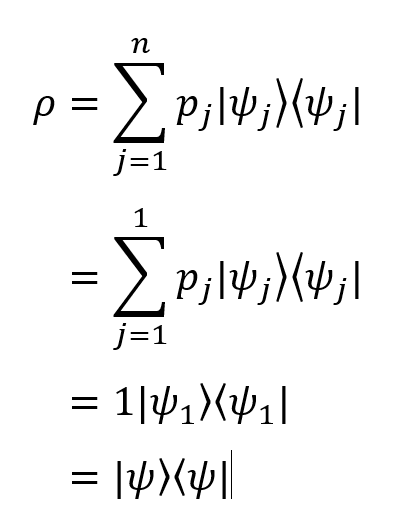
Так мы получаем второе, эквивалентное определение чистого состояния: состояние, в котором ρ = |ψ〉〈ψ| (то есть с матрицей плотности, состоящей из единственного проектора), является чистым.

Применим оператор плотности к нашему вектору чистого состояния:

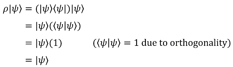
Как видите, в результате остается только |ψ〉.

По аналогии, вероятность обнаружить систему в некотором состоянии |φ〉 равна P = 〈φ|ρ|φ〉 = |〈φ|ψ〉|².

Как мы видим, правила вычисления вероятностей для смешанных состояний сводятся к правилам для чистых состояний, которые мы уже знаем. Таким образом, все правила для смешанных состояний выражаются через правила для чистых состояний, как и утверждалось ранее.

Дополнительные ресурсы

Microsoft Quantum
Microsoft Quantum Development Kit
Блог Microsoft Quantum

Источник

Плотность состояний

Предмет
Материаловедение

Разместил

🤓 comenvidu1988829

👍 Проверено Автор24

число энергетических уровней, приходящихся на единичный энергетический интервал; используется в зонной теории электронов для описания распределения электронов по энергиям.

Научные статьи на тему «Плотность состояний»

Плотность вещества и формула плотности вещества

У вещества бывают разные степени плотности, если оно находится в различных агрегатных состояниях….
Иными словами, плотность вещества, находящегося в твердом состоянии, будет иным, чем плотность этого…
В замороженном состоянии вода (лед) будет иметь плотность уже 900 килограммов на кубический метр….
Значения по каждому веществу разделены на три составляющие:

плотность тела в твердом состоянии;
плотность…
тела в жидком состоянии;
плотность тела в газообразном состоянии.

Статья от экспертов

Плотность состояний двумерного нанокластера

Density of states of the 2D square N × N Al nanosystem are calculated on the base of the Hubbard model at atom numbers of N=3÷30. It is shown that the density of states essentially depends on the number of atoms at the small value of N and also on the location of an atom in the lattice. Density of states on the top and the edge tends to its value in the volume at the increase of TV. The system temperature was considered by the giving of hopping energy in the initial Hamiltonian.

Конденсация, формулы конденсации

Плотность насыщенного пара растет с увеличением температуры….
Состояние насыщенного пара….
силы давления, которые стремились бы уменьшить эту плотность….
Поэтому в критическом состоянии флуктуации плотности велики….
При этом формируется состояние подвижного равновесия фаз системы.

Статья от экспертов

Структуры зон и плотностей состояний антимонида индия

Впервые определены зоны и плотности состояний антимонида индия InSb с учетом и без учета спин-орбитального взаимодействия для многих направлений зоны Бриллюэна, в том числе с учетом остовных зон dи s-типа. Рассмотрены вклады состояний s-, p-, d-типа отдельно индия и сурьмы. Расчеты выполнены методом LAPW с обменно-корреляционным потенциалом в обобщенном градиентном приближении (LAPW + GGA). Установлены основные особенности влияния спин-орбитальной связи на электронную структуру кристалла InSb.

Повышай знания с онлайн-тренажером от Автор24!

Напиши термин
Выбери определение из предложенных или загрузи свое
Тренажер от Автор24 поможет тебе выучить термины с помощью удобных и приятных
карточек

Источник

Определение[править | править код]

Примеры[править | править код]

Использование[править | править код]

Внешние ссылки[править | править код]

Introduction[edit]

Definition[edit]

Symmetry[edit]

k-space topologies[edit]

Density of wave vector states (sphere)[edit]

Density of energy states[edit]

Dispersion relations[edit]

Isotropic dispersion relations[edit]

Parabolic dispersion[edit]

Linear dispersion[edit]

Distribution functions[edit]

Applications[edit]

Quantization[edit]

Photonic crystals[edit]

Computational calculation[edit]

Local density of states[edit]

Concept[edit]

A general definition[edit]

Solid state devices[edit]

Optics and photonics[edit]

See also[edit]

References[edit]

Further reading[edit]

External links[edit]

Основы квантовых вычислений: чистые и смешанные состояния

Статьи из цикла:

Чистые состояния

Смешанные состояния

Оператор плотности, ρ

Немного математики

Дополнительные ресурсы

Плотность состояний

Научные статьи на тему «Плотность состояний»

Плотность вещества и формула плотности вещества

Плотность состояний двумерного нанокластера

Конденсация, формулы конденсации

Повышай знания с онлайн-тренажером от Автор24!

Вам также может понравиться

Как найти потерянные документы на улице

Как найти скорость частицы в физике

Как найти утечку радиатора на

Добавить комментарий Отменить ответ