Как найти постоянный коэффициент

Ниже разберем способы, как решить линейные однородные и неоднородные дифференциальные уравнения порядка выше второго, имеющих постоянные коэффициенты. Подобные уравнения представлены записями y(n)+fn-1·y(n-1)+…+f1·y’+f0·y=0 и y(n)+fn-1·y(n-1)+…+f1·y’+f0·y=f(x), в которых f0, f1,…, fn-1 – являются действительными числами, а функция f(x) является непрерывной на интервале интегрирования X.

Оговоримся, что аналитическое решение подобных уравнений иногда неосуществимо, тогда используются приближенные методы. Но, конечно, некоторые случаи дают возможность определить общее решение.

Общее решение ЛОДУ и ЛДНУ

Мы зададим формулировку двух теорем, показывающих, какого вида общих решений ЛОДУ и ЛНДУ n-ого порядка следует искать.

Общим решением y0 ЛОДУ y(n)+fn-1·y(n-1)+…+f1·y’+f0·y=0 на интервале
X (коэффициенты f0(x), f1(x),…, fn-1(x) непрерывны на X) будет линейная комбинация
n линейно независимых частных решений ЛОДУ yj, j=1, 2,…, n, содержащая произвольные постоянные коэффициенты Cj, j=1, 2,…, n, то есть y0=∑j=1nCj·yj.

Общим решением y ЛНДУ y(n)+fn-1·y(n-1)+…+f1·y’+f0·y=f(x) на интервале X (коэффициенты f0(x), f1(x),…, fn-1(x) непрерывны на X )  и функцией f(x) будет являться сумма y=y0+y~, где y0 – общее решение соответствующего ЛОДУ y(n)+fn-1·y(n-1)+…+f1·y’+f0·y=0, а y~ – некоторое частное решение исходного ЛНДУ.

Итак, общее решение линейного неоднородного дифференциального уравнения, содержащего постоянные коэффициенты y(n)+fn-1·y(n-1)+…+f1·y’+f0·y=f(x), нужно искать, как y=y0+y~, где y~ – некоторое его частное решение, а y0=∑j=1nCj·yj – общее решение соответствующего однородного дифференциального уравнения y(n)+fn-1·y(n-1)+…+f1·y’+f0·y=0.

В первую очередь рассмотрим, как осуществлять нахождение y0=∑j=1nCj·yj – общее решение ЛОДУ n-ого порядка с постоянными коэффициентами, а потом научимся определять частное решение y~ линейного неоднородного дифференциального уравнения n-ого порядка при постоянных коэффициентах.

Алгебраическое уравнение n-ого порядка kn+fn-1·kn-1+…+f1·k+f0=0 носит название характеристического уравнения линейного однородного дифференциального уравнения n-ого порядка, содержащего постоянные коэффициенты,  записи y(n)+fn-1·y(n-1)+…+f1·y’+f0·y=0.

Возможно определить n частных линейно независимых решений y1, y2,…, yn исходного ЛОДУ, исходя из значений найденных n корней характеристического уравнения k1, k2,…, kn.

Методы решения ЛОДУ и ЛНДУ

Укажем все существующие варианты и приведем примеры на каждый.

1. Когда все решения k1, k2,…, kn характеристического уравнения kn+fn-1·kn-1+…+f1·k+f0=0 действительны и различны, линейно независимые частные решения будут выглядеть так:
   y1=ek1·x, y2=ek2·x,…, yn=ekn·x. Общее же решение ЛОДУ n-ого порядка при постоянных коэффициентах запишем как: y0=C1·ek1·x+C2·ek2·x+…+Cn·ekn·x.

1. Когда решения характеристического уравнения являются действительными и одинаковыми ( k1=k2=…=kn=k0), линейно независимые частные решения линейного однородного дифференциального уравнения n-ого порядка с постоянными коэффициентами буду иметь вид: y1=ek0·x, y2=x·ek0·x,…, yn=xn-1·ek0·x.

Общее же решение ЛОДУ будет выглядеть так:
 y0=C1·ek0·x+C2·ek0·x+…+Cn·xn-1·ek0·x==ek0·x·C1+C2·x+…+Cn·xn-1

1. Когда решения характеристического уравнения линейного однородного дифференциального уравнения n-ого порядка при постоянных коэффициентах –  различные комплексно сопряженные пары α1±i·β1, α2±i·β2,…, αm±i·βm, n=2m, линейно независимые частные решения такого ЛОДУ будут иметь вид:
   y1=eα1x·cos β1x, y2=eα1x·sin β1x,y3=eα2x·cos β2x, y4=eα2x·sin β2x,…yn-1=eαmx·cos βmx, yn=eαmx·sin βmx

Общее же решение запишем так:

y0=eα1x·C1·cosβ1x+C2·sinβ1x++eα2x·C3·cosβ2x+C4·sinβ2x+…++eαmx·Cn-1·cosβmx+Cn·sinβmx

1. Когда решения характеристического уравнения – это совпадающие комплексно сопряженные пары α±i·β,  линейно независимыми частными решениями линейного однородного дифференциального уравнения n-ого порядка с постоянными коэффициентами будут записи:
   y1=eα·x·cos β x, y2=eα·x·sin β x,y3=eα·x·x·cos β x, y4=eα·x·x·sin β x,…yn-1=eα·x·xm-1·cos β x, yn=eα·x·xm-1·sin β x

Общим решением ЛОДУ будет:

y0=eα·x·C1·cosβ x+C2·sinβ x++eα·x·x·C4·cosβ x+C3·sinβ x+…++eα·x·xm-1·Cn-1·cosβ x+Cn·sinβ x==eα·x·cosβ x·C1+C3·x+…+Cn-1·xm-1++eα·x·sin β x·C2+C4·x+…+Cn·xm-1

1. Встречаются различные комбинации указанных случаев: некоторые корни характеристического уравнения ЛОДУ n-ого порядка с постоянными коэффициентами являются действительными и различными, некоторые – действительными и совпадающими, а какие-то – комплексно сопряженными парами или совпадающими комплексно сопряженными парами.

Таким образом, мы рассмотрели основные случаи, когда возможно определить y0 – общее решение ЛОДУ n-ого порядка с постоянными коэффициентами.

Следующее, что мы разберем – это ответ на вопрос, как решить линейное неоднородное дифференциальное уравнение n-ого порядка с постоянными коэффициентами записи y(n)+fn-1·y(n-1)+…+f1·y’+f0·y=f(x).

Общее решение в таком случае составляется как сумма общего решения соответствующего ЛОДУ и частного решения исходного ЛНДУ: y=y0+y~. Поскольку мы уже умеем определять y0, остается разобраться с нахождением y~, т.е. частного решения ЛНДУ порядка n с постоянными коэффициентами.

Приведем все способы нахождения y~ согласно тому, какой вид имеет функция f(x), находящаяся в правой части рассматриваемого ЛНДУ.

1. Когда  f(x) представлена в виде многочлена n-ой степени f(x) = Pn(x), частным решением ЛНДУ станет: y~=Qn(x)·xγ. Здесь Qn(x) является многочленом степени n, а r – указывает, сколько корней характеристического уравнения равно нулю.
2. Когда функция f(x) представлена в виде произведения многочлена степени n и экспоненты f(x)=Pn(x)·eα·x, частным решением ЛНДУ второго порядка станет: y~=eα·x·Qn(x)·xγ. Здесь Qn(x) является многочленом n-ой степени, r указывает, сколько корней характеристического уравнения равно α.
3. Когда функция f(x) записана как f(x)=A1cos(βx)+B1sin(βx), где А1 и В1 – числа, частным решением ЛНДУ станет запись y~=Acosβx+Bsinβx·xγ. Здесь где А и В являются неопределенными коэффициентами, r – указывает, сколько комплексно сопряженных пар корней характеристического уравнения равно ±iβ.
4. Когда f(x)=eαx·Pn(x)sinβx+Qkxcosβx, то y~=eαx·Lmxsinβx+Nmxcosβx·xγ, где r – указывает, сколько комплексно сопряженных пар корней характеристического уравнения равно α±iβ, Pn(x), Qk(x), Lm(x) и Nm(x) являются многочленами степени n, k, m и m соответственно, m=max(n,k).

Коэффициенты, которые неизвестны, определяются из равенства y~(n)+fn-1·y~(n-1)+…+f1y~’+f0·y~=f(x)

Подробности нахождения решений уравнений в каждом из указанных случаев можно изучить в статье линейные неоднородные дифференциальные уравнения второго порядка с постоянными коэффициентами, поскольку схемы решения ЛНДУ степени выше второй полностью совпадают.

Когда функция f(x) имеет любой иной вид, общее решение ЛНДУ возможно определить, используя метод вариации произвольных постоянных. Его разберем подробнее.

Пусть нам заданы yj, j=1,2,…, n – n линейно независимые частные решения соответствующего ЛОДУ, тогда, используя различные вариации произвольных постоянных, общим решением ЛНДУ
n-ого порядка с постоянными коэффициентами будет запись: н=∑j=1nCj(x)·yj. В нахождении производных функций Cj(x), j=1, 2,…, n поможет система уравнений:

∑j=1nCj'(x)·yj=0∑j=1nCj'(x)·y’j=0∑j=1nCj'(x)·y”j=0…∑j=1nCj'(x)·yj(n-2)=0∑j=1nCj'(x)·yj(n-1)=0

а собственно функции Cj(x), j=1, 2,…, n найдем при последующем интегрировании.

Разберем пример.

Линейная
однородная система с постоянными
коэффициентами
имеет вид

(22)

где
постоянные действительные числа. В
матричном виде система записывается
так:

(23)

где
Будем рассуждать так же, как при решении
однородных уравнений с постоянными
коэффициентами, т.е. попробуем найти
решения вида(постоянный вектор,постоянное число), а затем из этих решений
составить общее решение системы.
Продифференцируем функциюПодставим это выражение в уравнение
(23):Сократив набудем иметь:Это равенство означает, чтособственный
вектор
матрицы
аеёсобственное
значение.
Как известно из линейной алгебры,
собственные значения матрицы могут
быть найдены из характеристического
уравнения

(24)

где
единичная-матрица,
а собственные векторы находятся мз
системы линейных уравнений

(25)

Уравнение
(24) и систему (25) можно записать в
развёрнутом виде:

(26)

(27)

Предположим,
что имеет место “самый хороший” случай:
корни
характеристического уравнения
действительны и различны.
В этом случае, решив для каждого
систему уравнений (27), мы получимлинейно независимых собственных векторовЭти векторы определяютлинейно независимых вектор-функцийявляющихся решениями системы (22), а
значит, образующими фундаментальную
систему решений этой системы. Таким
образом, общее решение системы (22) имеет
вид

(28)

где
произвольные постоянные. Рассмотрим
пример.

Пример
1. Система

Найдём
все решения этой системы. Вначале запишем
эту систему в матричном виде:
Составим характеристическое уравнение:Имеем:откудаНайдём теперь собственные векторы. Длянадо решить системуа длярешить системуРешением первой системы будет вектора второй системы – векторИз формулы (28) получаем формулу общего
решения нашей системы:

где
произвольные постоянные. От векторной
формы общего решения можно перейти к
обычной форме:

Предположим,
что характеристическое уравнение имеет
кратный
корень
В этом случае, как и в случае простых
корней, мы находим собственные векторы
из системы (27), и если окажется, что
существуетлинейно независимых собственных
векторов, то общее решение системы также
запишется в виде (28). Если же собственных
векторов “не хватает” до базиса
пространствато можно искать решения системы в видеи т.д. Для матриц больших размеров такой
метод является неприемлемым, и
фундаментальную систему решений системы
(23) находят, приводя матрицукжордановой
нормальной форме.
Мы этот метод рассматривать не будем,
а ограничимся матрицами небольших
размеров.

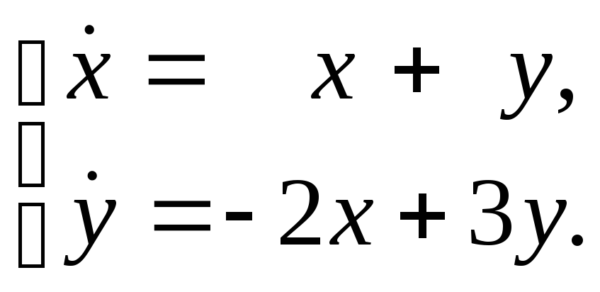
Пример
2. Система

Найдём
все решения этой системы. Характеристическое
уравнение

имеет
корни
Для собственных векторов смы имеем системуиз которой находим два линейно независимых
собственных вектора:иСобственные векторы, соответствующиенаходятся из системыПолучим:Так как векторылинейно независимы, то мы можем с их
помощью записать общее решение системы:

Пример
3. Система

Характеристическое
уравнение
имеет корниДля собственных векторов смы имеем системуиз которой находим векторДляимеем системурешения которой имеют видгдеСобственные векторыне составляют базиса пространстваПоэтому будем искать решения системы
дифференциальных уравнений, имеющие
видгдепостоянные векторы. В нашем примерено мы проделаем выкладки для произвольногоИмеем:Подставим в систему дифференциальных
уравнений:Отсюда следует, что

Таким
образом,
собственный вектор. Векторудовлетворяющий уравнениюв линейной алгебре называюткорневым
вектором.
В нашем примере
а для векторамы имеем системут.е.Этой системе удовлетворяет, например,
векторЗначит,ещё одно решение системы дифференциальных
уравнений. Итак, теперь найдены три
линейно независимых решения системы
дифференциальных уравнений, поэтому
мы можем написать её общее решение:

Наконец,
выясним, как найти решения системы (23),
соответствующие комплексным
собственным значениям матрицы А.
Пусть
комплексный корень характеристического
уравнения, асоответствующий ему собственный вектор.
Имеем:Тогдакомплексное решение системы (23). Пустьгдедействительные вектор-функции. Так кактои мы получаем:иТаким образом, вектор-функцииитоже решения системы.

Проиллюстрируем
эти рассуждения примером.

Пример
4. Система

Чтобы
решить систему, вначале составим
характеристическое уравнение:
Отсюдаа значит,Собственный вектор, соответствующий
собственному значениюнайдём из системыт.е.Решив систему, получим:Следовательно,комплексное решение системы. Отделим
в вектор-функциидействительную часть от мнимой:

Отсюда
получаем:
и мы можем выписать общее решение
системы:

Подведём
итог рассуждениям этого параграфа,
сформулировав теорему. Недоказанным в
этой теореме останется лишь утверждение
(г) и метод нахождения решений в случае
отсутствия базиса из собственных
векторов. Эти недостающие детали можно
найти в более подробных учебниках по
дифференциальным уравнениям.

Теорема.
Решения системы дифференциальных
уравнений
с постоянными коэффициентами могут
быть получены следующим образом:

(а)
если корни
характеристического уравнениядействительны и различны, то общее
решение системы имеет вид

где
собственные векторы, соответствующие
собственным значениямапроизвольные постоянные;

(б)
если корни характеристического уравнения

действительные, не обязательно различные,
но существует базиспространствасостоящий из собственных векторов
(соответствующих числам),
то также

(в)
если
комплексный корень характеристического
уравнения исоответствующий собственный вектор,
то вектор-функциииявляются решениями системы дифференциальных
уравнений;

(г)
если
кратный корень характеристического
уравнения, то ему соответствует решение
системы, имеющее вида есликомплексный корень, то следует взятьи

Соседние файлы в папке Прокофьев

• #
• #
• #
• #
• #
• #
• #

Постоянный коэффициент

Cтраница 1

Постоянный коэффициент е в правой части уравнения ( 83) имеет размерность 1 / с. Его называют скоростью разгона объекта, под которой понимается скорость изменения выходной величины ф при предварительном скачкообразном изменении входной величины ц, равном единице.
 [1]

Постоянный коэффициент Т0 при первой производной в левой части уравнений ( 95) и ( 96) имеет размерность времени и называется постоянной времени. Под постоянной времени объекта понимается время, в течение которого параметр объекта в случае скачкообразного возмущения достигнет нового равновесного состояния при условии, что параметр изменяется с постоянной скоростью, равной скорости в момент возмущения.
 [2]

Постоянные коэффициенты этой функции определяются экспериментально. Многие гиперупругие тела незначительно изменяют свой объем при деформировании.
 [3]

Постоянный коэффициент kw в формуле (4.12) обычно называют ветровым коэффициентом и принимают равным отношению скорости поверхностного течения к скорости ветра. Числовое значение kw получают как среднее арифметическое из большого количества результатов произведенных в натуре измерений.
 [4]

Постоянные коэффициенты С зависят только от отношения с толщины стенки к диаметру оболочки и могут быть найдены без особых трудностей ( многие из этих – коэффициентов равны нулю) путем подстановки упомянутых выше представлений для перемещений в основные уравнения, приведения подобных членов и решения пблучающихся в результате алгебраических уравнений.
 [5]

Постоянный коэффициент 48 80 был выведен как теплота полного сгорания угля, считая на один грамматом кислорода, а коэффициент 10 60 – как теплота конденсации образующихся водяных паров в жидкую воду.
 [6]

Постоянные коэффициенты здесь имеют размерность сопротивлений и поэтому данная система уравнений называется системой г-параметров.
 [8]

Постоянный коэффициент г, характерный для данного вещества, называют удельной рефракцией.
 [9]

Постоянные коэффициенты В, С и D должны определяться из экспериментальных данных.
 [10]

Постоянные коэффициенты Ь0 ется следующим образом.
 [12]

Постоянные коэффициенты V0 и m определяются по двум точкам а и б, произвольно взятым на прямолинейной части графика ( см. рис. VII.
 [13]

Постоянные коэффициенты at, bt и с / определяются из условия наибольшего соответствия формулы заданному участку характеристики. Если переходный процесс происходит на некоторой ветви частного цикла перемагничивания, то в аналитическое выражение необходимо ввести постоянную составляющую тока или магнитного потока.
 [14]

Постоянный коэффициент К имеет размерность расстояния и называется длиной волны. Если мысленно представить себе электромагнитное поле застывшим во времени, то его изменение по дальности будет происходить с периодом К, то есть вдоль направления распространения поле имеет волновой характер.
 [15]

Страницы:  

   1

   2

   3

   4