Вектор Пойнтинга в физике, теория и онлайн калькуляторы
Вектор Пойнтинга (вектор Умова – Пойнтинга)
Перенос энергии бегущей упругой и электромагнитной волной определяют при помощи вектора, который называют вектором потока энергии. Этот вектор обозначим как $overline{S} $(встречается обозначение $overline{P}$) Он показывает количество энергии, протекающее в волне за единицу времени через единицу площади поперечного сечения волны. Для электромагнитных волн данный вектор был введен Пойнтингом в 1884 г. Скорость переноса энергии при помощи вектора Пойнтинга не изменяется и равна характеристической скорости распространения электромагнитной волны в пространстве. Сейчас данный вектор ($overline{S}$) называют вектором Умова – Пойнтинга.
Определение
Определение
Вектором Умова – Пойнтинга ($overline{S}$) называют физическую величину, определяющую поток энергии электромагнитного поля, который равен:
[overline{S}=left[overline{E}overline{H}right]left(1right),]
где $overline{E}$ – напряженность электрического поля; $overline{H}$ – напряженность магнитного поля. Направлен $overline{S}$ перпендикулярно $overline{E}$ и $overline{H}$ и совпадает с направлением распространения электромагнитной волны.
Величина вектора Умова – Пойнтинга
Правая часть формулы (1) представляет собой векторное произведение векторов, значит, величина вектора Умова – Пойнтинга для электромагнитной волны равна:
[S=EH{sin alpha } left(2right),]
где $alpha $ – угол между векторами $overline{E}$ и $overline{H}$, но $overline{E}bot $ $overline{H}$, следовательно, получаем для электромагнитной волны:
[S=EHleft(3right).]
Вектор $overline{S} $удовлетворяет в свободном пространстве уравнению непрерывности:
[div overline{S}+frac{partial w}{partial t}=0 left(4right),]
где $w$ – объемная плотность энергии электромагнитного поля.
Вектор Умова – Пойнтинга плоской электромагнитной волны
В случае плоской электромагнитной волны величина вектора $overline{S}$ равна:
[P=frac{E^2}{mu {mu }_0u}left(5right),]
где $u$ $=frac{1}{sqrt{{mu }_0mu varepsilon {varepsilon }_0}}$- фазовая скорость распространения электромагнитного возмущения в веществе с диэлектрической проницаемостью $varepsilon $ и магнитной проницаемостью $mu .$
[u=frac{c}{sqrt{varepsilon mu }} left(6right),]
где $c$ – скорость света в вакууме.
Мгновенные величины напряженности магнитного и электрического полей в рассматриваемой волне связаны соотношением:
[sqrt{{varepsilon varepsilon }_0}E=sqrt{mu {mu }_0}Hleft(7right),]
выразим напряженность $H$:
[H=frac{sqrt{{varepsilon varepsilon }_0}E}{sqrt{mu {mu }_0}}(8).]
Учитывая формулу (8) величину вектора $overline{S}$ запишем как:
[S=varepsilon {varepsilon }_0uE^2left(9right).]
В изотропном веществе объемную плотность энергии электромагнитного поля найдем как:
[w=frac{1}{2}left(overline{E}overline{D}+overline{B}overline{H}right)=ее_0=mu {mu }_0H^2=frac{sqrt{varepsilon mu }EH}{c}left(10right).]
Учитывая формулы (6) и (10) запишем еще одно выражение для величины вектора $overline{S}$:
[S=uwleft(11right).]
На практике переходят от мгновенных величин к их средним значениям. Для плоской электромагнитной волны средняя величина по времени вектора Умова – Пойнтинга равна:
[{leftlangle Srightrangle }_t=frac{uvarepsilon {varepsilon }_0E^2}{2}(12).]
Модуль величины $left|{leftlangle Srightrangle }_tright|$ называют интенсивностью ($I$) электромагнитной волны:
[I=left|{leftlangle Srightrangle }_tright|=uleftlangle wrightrangle left(13right).]
Направление вектора Умова – Пойнтинга показывает направление движения энергии в электромагнитном поле. Если изобразить линии, касательные к которым в любой точке совпадут с направлениями вектора $overline{S}$, то такие линии будут являться путями распространения энергии электромагнитного поля. В оптике это лучи.
Примеры задач с решением
Пример 1
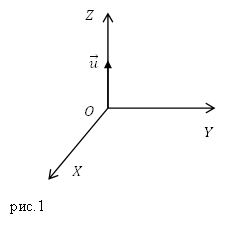
Задание. На рис.1 изображен вектор фазовой скорости плоской электромагнитной волны. В какой плоскости расположены векторы $overline{E}$ и $overline{H}$ полей этой волны?
Решение. Основой решения нашей задачи будем считать определение вектора $overline{S}$:
[overline{S}=left[overline{E}overline{H}right]left(1.1right).]
Вектор $overline{S}$ является результатом векторного произведения векторов$overline{E}$ и $overline{H}$, он направлен в сторону распространения электромагнитной волны, следовательно, $overline{S}uparrow uparrow overline{v}$, для рис.1 вектор Умова – Пойнтинга направлен по оси Z. Значит, векторы $overline{E }и overline{H}$ лежат в плоскости XOY.
Ответ. XOY
Пример 2
Задание. Запишите модуль среднего вектора Умова – Пойнтинга электромагнитной волны: $overline{E}=E_0{cos left(omega t-kxright). } $Считайте, что волна распространяется в вакууме по оси X.
Решение. Модуль вектора Умова – Пойнтинга для электромагнитной волны:
[S=EHleft(2.1right),]
где $E$ и $H$ – мгновенные значения электрического и магнитного полей. Мгновенное значение вектора Умова – Пойнтинга будет равно:
[S=EH=E_0H_0{{cos}^2 left(omega t-kxright)(2.2), }]
где $H_0$ – амплитуда колебаний напряженности магнитного поля.
Средняя величина ${leftlangle Srightrangle }_t$ может быть найдена:
[{leftlangle Srightrangle }_t=frac{E_0H_0}{2}left(2.3right),]
принимая во внимание, что ${leftlangle {{cos}^2 left(omega t-kxright) }rightrangle }_t=frac{1}{2}$, для вакуума имеем:
[sqrt{{varepsilon }_0}E=sqrt{{mu }_0}Hto H_0=frac{sqrt{{varepsilon }_0}E_0}{sqrt{{mu }_0}}left(2.4right).]
Подставим результат (2.4) в (2.3), тогда:
[{leftlangle Srightrangle }_t=frac{{E_0}^2}{2}frac{sqrt{{varepsilon }_0}}{sqrt{{mu }_0}}.]
Ответ. ${leftlangle Srightrangle }_t=sqrt{frac{{varepsilon }_0}{{mu }_0}}frac{{E_0}^2}{2}$
Читать дальше: вектор электрической индукции.

236
проверенных автора готовы помочь в написании работы любой сложности
Мы помогли уже 4 396 ученикам и студентам сдать работы от решения задач до дипломных на отлично! Узнай стоимость своей работы за 15 минут!
Dipole radiation of a dipole vertically in the page showing electric field strength (color) and Poynting vector (arrows) in the plane of the page.
In physics, the Poynting vector (or Umov–Poynting vector) represents the directional energy flux (the energy transfer per unit area per unit time) or power flow of an electromagnetic field. The SI unit of the Poynting vector is the watt per square metre (W/m2); kg/s3 in base SI units. It is named after its discoverer John Henry Poynting who first derived it in 1884.[1]: 132 Nikolay Umov is also credited with formulating the concept.[2] Oliver Heaviside also discovered it independently in the more general form that recognises the freedom of adding the curl of an arbitrary vector field to the definition.[3] The Poynting vector is used throughout electromagnetics in conjunction with Poynting’s theorem, the continuity equation expressing conservation of electromagnetic energy, to calculate the power flow in electromagnetic fields.
Definition[edit]
In Poynting’s original paper and in most textbooks, the Poynting vector 

where bold letters represent vectors and
- E is the electric field vector;
- H is the magnetic field’s auxiliary field vector or magnetizing field.
This expression is often called the Abraham form and is the most widely used.[7] The Poynting vector is usually denoted by S or N.
In simple terms, the Poynting vector S depicts the direction and rate of transfer of energy, that is power, due to electromagnetic fields in a region of space that may or may not be empty. More rigorously, it is the quantity that must be used to make Poynting’s theorem valid. Poynting’s theorem essentially says that the difference between the electromagnetic energy entering a region and the electromagnetic energy leaving a region must equal the energy converted or dissipated in that region, that is, turned into a different form of energy (often heat). So if one accepts the validity of the Poynting vector description of electromagnetic energy transfer, then Poynting’s theorem is simply a statement of the conservation of energy.
If electromagnetic energy is not gained from or lost to other forms of energy within some region (e.g., mechanical energy, or heat), then electromagnetic energy is locally conserved within that region, yielding a continuity equation as a special case of Poynting’s theorem:

where 
Example: Power flow in a coaxial cable[edit]
Although problems in electromagnetics with arbitrary geometries are notoriously difficult to solve, we can find a relatively simple solution in the case of power transmission through a section of coaxial cable analyzed in cylindrical coordinates as depicted in the accompanying diagram. We can take advantage of the model’s symmetry: no dependence on θ (circular symmetry) nor on Z (position along the cable). The model (and solution) can be considered simply as a DC circuit with no time dependence, but the following solution applies equally well to the transmission of radio frequency power, as long as we are considering an instant of time (during which the voltage and current don’t change), and over a sufficiently short segment of cable (much smaller than a wavelength, so that these quantities are not dependent on Z). The coaxial cable is specified as having an inner conductor of radius R1 and an outer conductor whose inner radius is R2 (its thickness beyond R2 doesn’t affect the following analysis). In between R1 and R2 the cable contains an ideal dielectric material of relative permittivity εr and we assume conductors that are non-magnetic (so μ = μ0) and lossless (perfect conductors), all of which are good approximations to real-world coaxial cable in typical situations.

Illustration of electromagnetic power flow inside a coaxial cable according to the Poynting vector S, calculated using the electric field E (due to the voltage V) and the magnetic field H (due to current I).

DC power transmission through a coaxial cable showing relative strength of electric (


The center conductor is held at voltage V and draws a current I toward the right, so we expect a total power flow of P = V · I according to basic laws of electricity. By evaluating the Poynting vector, however, we are able to identify the profile of power flow in terms of the electric and magnetic fields inside the coaxial cable. The electric fields are of course zero inside of each conductor, but in between the conductors (

W can be evaluated by integrating the electric field from 


so that:

The magnetic field, again by symmetry, can only be non-zero in the θ direction, that is, a vector field looping around the center conductor at every radius between R1 and R2. Inside the conductors themselves the magnetic field may or may not be zero, but this is of no concern since the Poynting vector in these regions is zero due to the electric field’s being zero. Outside the entire coaxial cable, the magnetic field is identically zero since paths in this region enclose a net current of zero (+I in the center conductor and −I in the outer conductor), and again the electric field is zero there anyway. Using Ampère’s law in the region from R1 to R2, which encloses the current +I in the center conductor but with no contribution from the current in the outer conductor, we find at radius r:

Now, from an electric field in the radial direction, and a tangential magnetic field, the Poynting vector, given by the cross-product of these, is only non-zero in the Z direction, along the direction of the coaxial cable itself, as we would expect. Again only a function of r, we can evaluate S(r):

where W is given above in terms of the center conductor voltage V. The total power flowing down the coaxial cable can be computed by integrating over the entire cross section A of the cable in between the conductors:

Substituting the earlier solution for the constant W we find:

that is, the power given by integrating the Poynting vector over a cross section of the coaxial cable is exactly equal to the product of voltage and current as one would have computed for the power delivered using basic laws of electricity.
Other forms[edit]
In the “microscopic” version of Maxwell’s equations, this definition must be replaced by a definition in terms of the electric field E and the magnetic flux density B (described later in the article).
It is also possible to combine the electric displacement field D with the magnetic flux B to get the Minkowski form of the Poynting vector, or use D and H to construct yet another version. The choice has been controversial: Pfeifer et al.[8] summarize and to a certain extent resolve the century-long dispute between proponents of the Abraham and Minkowski forms (see Abraham–Minkowski controversy).
The Poynting vector represents the particular case of an energy flux vector for electromagnetic energy. However, any type of energy has its direction of movement in space, as well as its density, so energy flux vectors can be defined for other types of energy as well, e.g., for mechanical energy. The Umov–Poynting vector[9] discovered by Nikolay Umov in 1874 describes energy flux in liquid and elastic media in a completely generalized view.
Interpretation[edit]
The Poynting vector appears in Poynting’s theorem (see that article for the derivation), an energy-conservation law:

where Jf is the current density of free charges and u is the electromagnetic energy density for linear, nondispersive materials, given by

where
- E is the electric field;
- D is the electric displacement field;
- B is the magnetic flux density;
- H is the magnetizing field.[10]: 258–260
The first term in the right-hand side represents the electromagnetic energy flow into a small volume, while the second term subtracts the work done by the field on free electrical currents, which thereby exits from electromagnetic energy as dissipation, heat, etc. In this definition, bound electrical currents are not included in this term and instead contribute to S and u.
For linear, nondispersive and isotropic (for simplicity) materials, the constitutive relations can be written as

where
- ε is the permittivity of the material;
- μ is the permeability of the material.[10]: 258–260
Here ε and μ are scalar, real-valued constants independent of position, direction, and frequency.
In principle, this limits Poynting’s theorem in this form to fields in vacuum and nondispersive[clarification needed] linear materials. A generalization to dispersive materials is possible under certain circumstances at the cost of additional terms.[10]: 262–264
One consequence of the Poynting formula is that for the electromagnetic field to do work, both magnetic and electric fields must be present. The magnetic field alone or the electric field alone cannot do any work.[11]
Plane waves[edit]
In a propagating electromagnetic plane wave in an isotropic lossless medium, the instantaneous Poynting vector always points in the direction of propagation while rapidly oscillating in magnitude. This can be simply seen given that in a plane wave, the magnitude of the magnetic field H(r,t) is given by the magnitude of the electric field vector E(r,t) divided by η, the intrinsic impedance of the transmission medium:

where |A| represents the vector norm of A. Since E and H are at right angles to each other, the magnitude of their cross product is the product of their magnitudes. Without loss of generality let us take X to be the direction of the electric field and Y to be the direction of the magnetic field. The instantaneous Poynting vector, given by the cross product of E and H will then be in the positive Z direction:

Finding the time-averaged power in the plane wave then requires averaging over the wave period (the inverse frequency of the wave):

where Erms is the root mean square electric field amplitude. In the important case that E(t) is sinusoidally varying at some frequency with peak amplitude Epeak, its rms voltage is given by 

This is the most common form for the energy flux of a plane wave, since sinusoidal field amplitudes are most often expressed in terms of their peak values, and complicated problems are typically solved considering only one frequency at a time. However, the expression using Erms is totally general, applying, for instance, in the case of noise whose RMS amplitude can be measured but where the “peak” amplitude is meaningless. In free space the intrinsic impedance η is simply given by the impedance of free space η0 ≈ 377 Ω. In non-magnetic dielectrics (such as all transparent materials at optical frequencies) with a specified dielectric constant εr, or in optics with a material whose refractive index 

In optics, the value of radiated flux crossing a surface, thus the average Poynting vector component in the direction normal to that surface, is technically known as the irradiance, more often simply referred to as the intensity (a somewhat ambiguous term).
Formulation in terms of microscopic fields[edit]
The “microscopic” (differential) version of Maxwell’s equations admits only the fundamental fields E and B, without a built-in model of material media. Only the vacuum permittivity and permeability are used, and there is no D or H. When this model is used, the Poynting vector is defined as

where
- μ0 is the vacuum permeability;
- E is the electric field vector;
- B is the magnetic flux.
This is actually the general expression of the Poynting vector[dubious – discuss].[12] The corresponding form of Poynting’s theorem is

where J is the total current density and the energy density u is given by

where ε0 is the vacuum permittivity. It can be derived directly from Maxwell’s equations in terms of total charge and current and the Lorentz force law only.
The two alternative definitions of the Poynting vector are equal in vacuum or in non-magnetic materials, where B = μ0H. In all other cases, they differ in that S = (1/μ0) E × B and the corresponding u are purely radiative, since the dissipation term −J ⋅ E covers the total current, while the E × H definition has contributions from bound currents which are then excluded from the dissipation term.[13]
Since only the microscopic fields E and B occur in the derivation of S = (1/μ0) E × B and the energy density, assumptions about any material present are avoided. The Poynting vector and theorem and expression for energy density are universally valid in vacuum and all materials.[13]
Time-averaged Poynting vector[edit]
The above form for the Poynting vector represents the instantaneous power flow due to instantaneous electric and magnetic fields. More commonly, problems in electromagnetics are solved in terms of sinusoidally varying fields at a specified frequency. The results can then be applied more generally, for instance, by representing incoherent radiation as a superposition of such waves at different frequencies and with fluctuating amplitudes.
We would thus not be considering the instantaneous E(t) and H(t) used above, but rather a complex (vector) amplitude for each which describes a coherent wave’s phase (as well as amplitude) using phasor notation. These complex amplitude vectors are not functions of time, as they are understood to refer to oscillations over all time. A phasor such as Em is understood to signify a sinusoidally varying field whose instantaneous amplitude E(t) follows the real part of Em ejωt where ω is the (radian) frequency of the sinusoidal wave being considered.
In the time domain, it will be seen that the instantaneous power flow will be fluctuating at a frequency of 2ω. But what is normally of interest is the average power flow in which those fluctuations are not considered. In the math below, this is accomplished by integrating over a full cycle T = 2π / ω. The following quantity, still referred to as a “Poynting vector”, is expressed directly in terms of the phasors as:

where ∗ denotes the complex conjugate. The time-averaged power flow (according to the instantaneous Poynting vector averaged over a full cycle, for instance) is then given by the real part of Sm. The imaginary part is usually ignored, however, it signifies “reactive power” such as the interference due to a standing wave or the near field of an antenna. In a single electromagnetic plane wave (rather than a standing wave which can be described as two such waves travelling in opposite directions), E and H are exactly in phase, so Sm is simply a real number according to the above definition.
The equivalence of Re(Sm) to the time-average of the instantaneous Poynting vector S can be shown as follows.

The average of the instantaneous Poynting vector S over time is given by:
![{displaystyle langle mathbf {S} rangle ={frac {1}{T}}int _{0}^{T}mathbf {S} (t),dt={frac {1}{T}}int _{0}^{T}!left[{tfrac {1}{2}}operatorname {Re} !left(mathbf {E} _{mathrm {m} }times mathbf {H} _{mathrm {m} }^{*}right)+{tfrac {1}{2}}operatorname {Re} !left({mathbf {E} _{mathrm {m} }}times {mathbf {H} _{mathrm {m} }}e^{2jomega t}right)right]dt.}](https://wikimedia.org/api/rest_v1/media/math/render/svg/9d6783ee9e038080c9c4768c26588ac2a5f25e9f)
The second term is the double-frequency component having an average value of zero, so we find:

According to some conventions, the factor of 1/2 in the above definition may be left out. Multiplication by 1/2 is required to properly describe the power flow since the magnitudes of Em and Hm refer to the peak fields of the oscillating quantities. If rather the fields are described in terms of their root mean square (RMS) values (which are each smaller by the factor 
Resistive dissipation[edit]
If a conductor has significant resistance, then, near the surface of that conductor, the Poynting vector would be tilted toward and impinge upon the conductor. Once the Poynting vector enters the conductor, it is bent to a direction that is almost perpendicular to the surface.[14]: 61 This is a consequence of Snell’s law and the very slow speed of light inside a conductor. The definition and computation of the speed of light in a conductor can be given.[15]: 402 Inside the conductor, the Poynting vector represents energy flow from the electromagnetic field into the wire, producing resistive Joule heating in the wire. For a derivation that starts with Snell’s law see Reitz page 454.[16]: 454
Radiation pressure[edit]
The density of the linear momentum of the electromagnetic field is S/c2 where S is the magnitude of the Poynting vector and c is the speed of light in free space. The radiation pressure exerted by an electromagnetic wave on the surface of a target is given by

Uniqueness of the Poynting vector[edit]
The Poynting vector occurs in Poynting’s theorem only through its divergence ∇ ⋅ S, that is, it is only required that the surface integral of the Poynting vector around a closed surface describe the net flow of electromagnetic energy into or out of the enclosed volume. This means that adding a solenoidal vector field (one with zero divergence) to S will result in another field that satisfies this required property of a Poynting vector field according to Poynting’s theorem. Since the divergence of any curl is zero, one can add the curl of any vector field to the Poynting vector and the resulting vector field S′ will still satisfy Poynting’s theorem.
However even though the Poynting vector was originally formulated only for the sake of Poynting’s theorem in which only its divergence appears, it turns out that the above choice of its form is unique.[10]: 258–260, 605–612 The following section gives an example which illustrates why it is not acceptable to add an arbitrary solenoidal field to E × H.
Static fields[edit]
Poynting vector in a static field, where E is the electric field, H the magnetic field, and S the Poynting vector.
The consideration of the Poynting vector in static fields shows the relativistic nature of the Maxwell equations and allows a better understanding of the magnetic component of the Lorentz force, q(v × B). To illustrate, the accompanying picture is considered, which describes the Poynting vector in a cylindrical capacitor, which is located in an H field (pointing into the page) generated by a permanent magnet. Although there are only static electric and magnetic fields, the calculation of the Poynting vector produces a clockwise circular flow of electromagnetic energy, with no beginning or end.
While the circulating energy flow may seem unphysical, its existence is necessary to maintain conservation of angular momentum. The momentum of an electromagnetic wave in free space is equal to its power divided by c, the speed of light. Therefore the circular flow of electromagnetic energy implies an angular momentum.[17] If one were to connect a wire between the two plates of the charged capacitor, then there would be a Lorentz force on that wire while the capacitor is discharging due to the discharge current and the crossed magnetic field; that force would be tangential to the central axis and thus add angular momentum to the system. That angular momentum would match the “hidden” angular momentum, revealed by the Poynting vector, circulating before the capacitor was discharged.
See also[edit]
- Wave vector
References[edit]
- ^ Stratton, Julius Adams (1941). Electromagnetic Theory (1st ed.). New York: McGraw-Hill. ISBN 978-0-470-13153-4.
- ^ “Пойнтинга вектор”. Физическая энциклопедия (in Russian). Retrieved 2022-02-21.
- ^ Nahin, Paul J. (2002). Oliver Heaviside: The Life, Work, and Times of an Electrical Genius of the Victorian Age. p. 131. ISBN 9780801869099.
- ^ Poynting, John Henry (1884). “On the Transfer of Energy in the Electromagnetic Field”. Philosophical Transactions of the Royal Society of London. 175: 343–361. doi:10.1098/rstl.1884.0016.
- ^ Grant, Ian S.; Phillips, William R. (1990). Electromagnetism (2nd ed.). New York: John Wiley & Sons. ISBN 978-0-471-92712-9.
- ^ Griffiths, David J. (2012). Introduction to Electrodynamics (3rd ed.). Boston: Addison-Wesley. ISBN 978-0-321-85656-2.
- ^ Kinsler, Paul; Favaro, Alberto; McCall, Martin W. (2009). “Four Poynting Theorems”. European Journal of Physics. 30 (5): 983. arXiv:0908.1721. Bibcode:2009EJPh…30..983K. doi:10.1088/0143-0807/30/5/007. S2CID 118508886.
- ^ Pfeifer, Robert N. C.; Nieminen, Timo A.; Heckenberg, Norman R.; Rubinsztein-Dunlop, Halina (2007). “Momentum of an Electromagnetic Wave in Dielectric Media”. Reviews of Modern Physics. 79 (4): 1197. arXiv:0710.0461. Bibcode:2007RvMP…79.1197P. doi:10.1103/RevModPhys.79.1197.
- ^ Umov, Nikolay Alekseevich (1874). “Ein Theorem über die Wechselwirkungen in Endlichen Entfernungen”. Zeitschrift für Mathematik und Physik. 19: 97–114.
- ^ a b c d Jackson, John David (1998). Classical Electrodynamics (3rd ed.). New York: John Wiley & Sons. ISBN 978-0-471-30932-1.
- ^ “K. McDonald’s Physics Examples – Railgun” (PDF). puhep1.princeton.edu. Retrieved 2021-02-14.
- ^ Zangwill, Andrew (2013). Modern Electrodynamics. Cambridge University Press. p. 508. ISBN 9780521896979.
- ^ a b Richter, Felix; Florian, Matthias; Henneberger, Klaus (2008). “Poynting’s Theorem and Energy Conservation in the Propagation of Light in Bounded Media”. EPL. 81 (6): 67005. arXiv:0710.0515. Bibcode:2008EL…..8167005R. doi:10.1209/0295-5075/81/67005. S2CID 119243693.
- ^ Harrington, Roger F. (2001). Time-Harmonic Electromagnetic Fields (2nd ed.). McGraw-Hill. ISBN 978-0-471-20806-8.
- ^ Hayt, William (2011). Engineering Electromagnetics (4th ed.). New York: McGraw-Hill. ISBN 978-0-07-338066-7.
- ^ Reitz, John R.; Milford, Frederick J.; Christy, Robert W. (2008). Foundations of Electromagnetic Theory (4th ed.). Boston: Addison-Wesley. ISBN 978-0-321-58174-7.
- ^ Feynman, Richard Phillips (2011). The Feynman Lectures on Physics. Vol. II: Mainly Electromagnetism and Matter (The New Millennium ed.). New York: Basic Books. ISBN 978-0-465-02494-0.
Further reading[edit]
![]()
- Becker, Richard (1982). Electromagnetic Fields and Interactions (1st ed.). Mineola, New York: Dover Publications. ISBN 978-0-486-64290-1.
- Edminister, Joseph; Nahvi, Mahmood (2013). Electromagnetics (4th ed.). New York: McGraw-Hill. ISBN 978-0-07-183149-9.

Виталий Викторович Карабут
Эксперт по предмету «Физика»
Задать вопрос автору статьи
Определение 1
Вектор потока электромагнитной энергии, определяемый как:
[overrightarrow{P}=left[overrightarrow{E}overrightarrow{H}right](1)]
называют вектором Умова – Пойнтинга (вектором Пойнтинга). Понятие вектора как потока энергии в разных веществах было введено Н.А. Умовым, а математическое выражение (1) получено Пойнтингом.
В электромагнитной волне векторы $overrightarrow{E } и overrightarrow{H}$ перпендикулярны, следовательно, модуль вектора $overrightarrow{P}$ имеет выражение:
Направление вектора Умова – Пойнтинга перпендикулярно к векторам $overrightarrow{E }и overrightarrow{H}$, и со направленно с направлением распространения волны ($overrightarrow{v}$).
Для плоской электромагнитной волны выражение для модуля вектора Умова – Пойнтинга имеет вид:
так как:
и между мгновенными значениями напряженности магнитного и электрического полей в электромагнитной волне существует соотношение:
откуда выражая напряженность магнитного поля, получаем:
Модуль вектора Умова — Пойнтинга можно выразить как:
В диэлектрике объемная плотность электромагнитного поля равна:
Следовательно, сравнивая равенства (6) и (7), имеем:
В уравнения (2) -(8) входят мгновенные значения величин. Векторы в световой волне совершают колебания с частотами около ${10}^{15}Гц$, следовательно, весьма затруднительно следить за изменением величин во времени. Поэтому обращаются к средним значениям, переходя от мгновенных величин. Если электромагнитная волна является плоской, то среднее значение по времени вектора Умова – Пойнтинга равно:
Вектор Умова – Пойнтинга связан с энергией, которую несет электромагнитная волна соотношением:
где $frac{partial W}{partial t}$ — энергия, проходящая через площадку $S$ в единицу времени, $P_n=Pcosalpha $ — проекция вектора $overrightarrow{P}$ на нормаль $overrightarrow{n}$ к площадке $S$. Направление вектора Умова – Пойнтинга дает характеристику движения энергии в электромагнитном поле.
«Вектор Умова-Пойнтинга» 👇
Определение 2
Если представить линии, касательные к которым в каждой точке совпадают с направлениями вектора $overrightarrow{P}$, то такие линии есть пути распространения энергии электромагнитного поля. В оптике подобные линии называют лучами.
Теорема Пойнтинга
Теорема 1
Для теории электромагнитных полей формулировки законов сохранения энергии и импульса имеет весьма важное значение. Теорема Пойнтинга – один из видов формулировок закона сохранения энергии: Скорость возрастания электромагнитной энергии внутри некоторого объема в сумме с энергией, которая вытекает за единицу времени через поверхность, ограничивающую тот же объем, равна полной работе, которую совершает поле над источниками внутри заданного объема, если взять ее со знаком минус.
Поясним данную формулировку. Выделим внутри некоторой среды объем $V$, который ограничивает поверхность $S$ (рис.1). Допустим, что полная энергия, которая заключена внутри объема, равна $W$. Тогда можно записать:
где $P_n$ — нормальная составляющая вектора Умова – Пойнтинга. Интегрирование в (4) производят по всей замкнутой поверхности $S$. Положительным считают направление внешней нормали $overrightarrow{n}$, что означает поток вектора $overrightarrow{P}$ (выражение, которое стоит в формуле (4) в правой части) считают большим нуля, если линии потока энергии $overrightarrow{P}$ выводят наружу из объема.
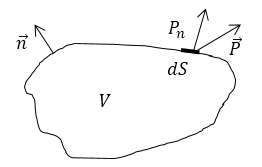
Рисунок 1.
При этом $-frac{partial W}{partial t}$- величина, на которую уменьшатся, полная энергия внутри объема $V$ за единицу времени. По закону сохранения энергии она должна быть равна энергии, которая выходит через поверхность $S$ за единицу времени наружу. Следовательно, энергия, покидающая объем $V$ через поверхность $S$, выражена потоком вектора Умова – Пойнтинга.
Пример 1
Задание: Напишите выражение для вектора Умова – Пойнтинга, если энергию переносит волна, уравнение изменения вектора напряженности электрического поля которой задано как: $overrightarrow{E}=10cosleft(omega t-kx+alpha right)overrightarrow{_z }(frac{В}{м}).$ Учесть, что амплитуда вектора напряженности магнитного поля имеет вид: $H_moverrightarrow{e_x}$, частота волны $omega при ней varepsilon =2, mu approx 1 .$
Решение:
За основу решения задачи, примем определение вектора Умова – Пойнтинга:
[overrightarrow{P}=left[overrightarrow{E}overrightarrow{H}right]left(1.1right).]
Из условий видим, что колебания вектора напряженности электрического поля происходят по $оси Z$, колебания вектора напряженности магнитного поля по $оси X$, следовательно, вектор Умова – Пойнтинга колеблется по $оси Y$.
Модуль искомого вектора можно найти как:
[P=EHleft(1.2right).]
Найдем амплитуду вектора $overrightarrow{H}$, если знаем, что амплитудные значения в нашем случае связаны соотношением:
[sqrt{varepsilon {varepsilon }_0}E_m=sqrt{mu {mu }_0}H_mleft(1.3right).]
Выразим из (1.3) искомую амплитуду $H_m$, имеем:
[H_m=sqrt{frac{varepsilon {varepsilon }_0}{mu {mu }_0}}E_mleft(1.4right).]
При этом уравнение колебаний вектора напряженности запишем в виде:
[overrightarrow{H}=sqrt{frac{varepsilon {varepsilon }_0}{mu {mu }_0}}E_mcosleft(omega t-kx+alpha right)overrightarrow{e_x }left(1.5right).]
Используя уравнения (1.1), (1.5) и уравнение колебаний вектора напряжённости электрического поля из условий задачи, запишем выражение для вектора Умова — Пойнтинга:
[P=sqrt{frac{varepsilon {varepsilon }_0}{mu {mu }_0}}{E_m}^2c{os}^2left(omega t-kx+alpha right)left(1.6right),]
где $varepsilon =2, mu =1, {varepsilon }_0=frac{1}{4pi cdot 9cdot {10}^9}frac{Ф}{м}, {mu }_0=4pi cdot {10}^{-7}frac{Н}{А^2}$, следовательно:
[{E_m}^2sqrt{frac{varepsilon {varepsilon }_0}{mu {mu }_0}}=100cdot sqrt{frac{2}{4pi cdot {10}^{-7}cdot 4pi cdot 9cdot {10}^9}}=0,37.]
Ответ: $overrightarrow{P}=sqrt{frac{varepsilon {varepsilon }_0}{mu {mu }_0}}{E_m}^2c{os}^2left(omega t-kx+alpha right)overrightarrow{e_y}.$
Пример 2
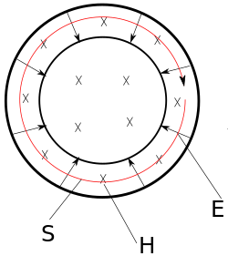
Задание: Плоский конденсатор, имеющий круглые обкладки заряжен постоянным током за время $t_0$ до напряжения $U$. Расстояние между пластинами конденсатора равно $d$. Запишите выражение для вектора Умова – Пойнтинга для точек воображаемой цилиндрической поверхности радиуса $r$, которая находится между обкладками конденсатора. Считайте, что радиус пластин конденсатора много больше, чем радиус воображаемого цилиндра.
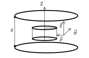
Рисунок 2.
Решение:
За основу решения задачи, примем определение вектора Умова — Пойнтинга:
[overrightarrow{P}=left[overrightarrow{E}overrightarrow{H}right]to P=EHleft(2.1right).]
Переменное электрическое поле, возникающее в результате разрядки конденсатора, вызывает переменное магнитное поле. Запишем уравнение из системы Максвелла, учитывая, что между обкладками конденсатора токов проводимости нет:
[rotoverrightarrow{H}=frac{partial overrightarrow{D}}{partial t}left(2.2right).]
и материальное уравнение:
[overrightarrow{D}=varepsilon {varepsilon }_0overrightarrow{E}={varepsilon }_0frac{U}{d}frac{t}{t_0}overrightarrow{e_z}left(2.3right).]
Возьмем производную от $overrightarrow{D}$ по времени:
[frac{partial overrightarrow{D}}{partial t}=varepsilon_0frac{U}{d}frac{1}{t_0}overrightarrow{e_z}=rotoverrightarrow{H}left(2.4right).]
Возьмём интеграл от $rotoverrightarrow{H}$ по поверхности цилиндра радиуса $r$, применим теорему Стокса:
[intlimits_S{rotoverrightarrow{H}doverrightarrow{S}}=intlimits_S{frac{partial overrightarrow{D}}{partial t}doverrightarrow{S}}=ointlimits_L{overrightarrow{H}doverrightarrow{l}left(2.5right),}]
где
[ointlimits_L{overrightarrow{H}doverrightarrow{l}=2pi rHleft(2.6right),}] [intlimits_S{frac{partial overrightarrow{D}}{partial t}doverrightarrow{S}}=varepsilon_0frac{U}{d}frac{1}{t_0}pi r^2left(2.7right).]
Приравняем правые части выражений (2.6), (2.7), согласно тому, что выполняется (2.5):
[2pi rH=varepsilon_0frac{U}{d}frac{1}{t_0}pi r^2to H=frac{varepsilon_0U}{2d}frac{r}{t_0}left(2.8right).]
Найдем модуль вектора Умова — Пойнтинга согласно выражениям (2.1) и (2.8):
[P=frac{U}{d}frac{t}{t_0}cdot frac{{varepsilon }_0U}{2d}frac{r}{t_0}=frac{{varepsilon }_0r}{2}frac{U^2}{d^2}frac{t}{{t_0}^2}.]
Ответ: $P=frac{varepsilon_0r}{2}frac{U^2}{d^2}frac{t}{{t_0}^2}.$
Пример 3
Задание: Плоская электромагнитная волна распространяется в вакууме по $оси X$. Чему равна средняя энергия, которая проходит через единицу поверхности в единицу времени?
Решение:
сли мы имеем плоскую электромагнитную волну, то модули напряженности полей $overrightarrow{E} $и $overrightarrow{H}$ в произвольной точке $x$ могут быть выражены как:
[E=E_0{sin left(omega t-kxright) }left(1.1right),] [H=H_0{sin left(omega t-kxright) }left(1.2right),]
где $k=frac{2pi }{lambda }$. Следовательно, мгновенное значение вектора $overrightarrow{P}$ можно записать в виде:
[P=E_0{H_0{sin}^2 left(omega t-kxright) }left(1.3right).]
По условию задачи волна распространяется в вакууме, следовательно, $varepsilon =1, mu =1 $, имеем следующее соотношение между амплитудами полей:
[sqrt{{varepsilon }_0}E_0=sqrt{{mu }_0}H_0left(1.4right).]
Кроме того, известно, что среднее значение $leftlangle {sin}^2alpha rightrangle =frac{1}{2},$ тогда используем (1.3), (1.4) получаем среднее значение вектора Умова – Пойнтинга ($leftlangle Prightrangle $) равно:
[leftlangle Prightrangle =sqrt{frac{{varepsilon }_0}{{mu }_0}}frac{E^2_0}{2}.]
Ответ: Средняя энергия, которая проходит через единицу поверхности за единицу времени (интенсивность волны), равна $leftlangle Prightrangle =sqrt{frac{{varepsilon }_0}{{mu }_0}}frac{E^2_0}{2}.$
Пример 4
Задание: Вычислите среднее значение вектора Умова – Пойнтинга в стоячей волне.
Решение:
Колебания электрического и магнитного полей можно представить в стоячей волне с использованием следующих гармонических законов:
[E=2E_0{cos left(kx-frac{{varphi }_E}{2}right) }{sin left(omega t-frac{{varphi }_E}{2}right) }left(2.1right),] [H=2H_0{cos left(kx-frac{{varphi }_H}{2}right) }{sin left(omega t-frac{{varphi }_H}{2}right) }left(2.2right),]
где ${varphi }_E, varphi_H$- запаздывание по фазе отраженной волны соответствующего поля, то есть:
[{varphi }_E=2pi frac{2l}{lambda }+theta (2.3),] [{varphi }_H=2pi frac{2l}{lambda }+ vartheta(2.4),]
здесь $theta ,vartheta $ – изменение фазы при отражении, они равны или $pi , $или 0. $l-$длина линии (если рассматривается свободная волна, то это расстояние от излучателя до поверхности отражения). Обозначим:
[2E_0{cos left(kx-frac{{varphi }_E}{2}right) }=E_1left(2.5right),] [2H_0{cos left(kx-frac{{varphi }_H}{2}right) }=H_1left(2.6right),]
тогда колебания, исходя из (2.1) и (2.2) в точке $x$ можно записать как:
[E=E_1{sin left(omega t-frac{{varphi }_E}{2}right) }left(2.7right),] [H=H_1{sin left(omega t-frac{{varphi }_H}{2}right) }left(2.8right),]
при этом очевидно, что $E_1$ и $H_1$ не зависят от времени. Допустим, что $theta =pi $, тогда:
[E=E_1{cos left(omega t-frac{2pi }{lambda }lright) }left(2.9right),] [H=H_1{sin left(omega t-frac{2pi }{lambda }lright) }left(2.10right).]
Исходя из (2.9) и (2.10), для вектора Умова – Пойнтинга получим:
[P=E_1{cos left(omega t-frac{2pi }{lambda }lright)H_1{sin left(omega t-frac{2pi }{lambda }lright) }=frac{E_1H_1}{2} }{sin left(2omega t-frac{4pi l}{lambda }right) }left(2.11right).]
Из формулы (2.11) следует, что колебания модуля вектора $overrightarrow{P}$ происходят с частотой $2omega $, при этом периодически изменяется знак. Следовательно, среднее значение вектора по времени равно $0$ ($leftlangle Prightrangle =0$).
Ответ: В стоячей волне течения энергии нет, $leftlangle Prightrangle =0$.
Находи статьи и создавай свой список литературы по ГОСТу
Поиск по теме
В
макроскопической электродинамике
система основных аксиом
уравнений Максвелла
дополняется двумя энергетическими
аксиомами:
1)
электромагнитная энергия распределена
в пространстве с объемной плотностью
![]()
,
Дж/м3,
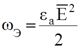
где
![]()
объемная плотность энергии электрического
поля;
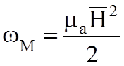
![]()
объемная плотность энергии магнитного
поля;
2)
величина и направление потока
электромагнитной энергии характеризуются
вектором Пойнтинга
![]()
.
С
учетом этого закон сохранения энергии
для электромагнитных процессов,
происходящих в некотором объеме
,
ограниченном поверхностью
(теорема
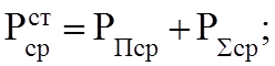
Пойнтинга), имеет следующий вид:
![]()
,
где
![]()
мощность сторонних сил;
![]()
мощность тепловых потерь;
![]()
электромагнитная энергия, запасенная
в обьеме
;
![]()
мощность, переносимая электромагнитным
полем через поверхность
;
![]()
вектор, по направлению совпадающий с
внешней нормалью;
внешняя нормаль к поверхности
.
Таким
образом, теорема Пойнтинга утверждает,
что мощность сторонних сил, действующих
в объеме
,
расходуется на тепловые потери, изменение
электромагнитной энергии и излучение
за пределы объема.
Отметим,
что слагаемые
![]()
и
![]()
могут быть как положительными, так
и отрицательными;
![]()
и
![]()
всегда положительны.
Для
полей, записанных в виде комплексных
амплитуд, вводится комплексный вектор
Пойнтинга
![]()
.
Среднее значение вектора Пойнтинга
![]()
,
где
период колебаний.
Аналогично
определяются средние значения и других
энергетических величин.
Задачи
5.1.
Вычислить энергию, запасенную в
плоском конденсаторе. Разность потенциалов
между пластинами
,
площадь
,
расстояние между пластинами
.
Поле считать однородным. Вывести
формулу для емкости конденсатора.
5.2.
Определить, с какой стороны к линии
подключены генератор и нагрузка,
объяснить полученный результат (рис.
5.1).
5.3.
Двухпроводная линия проходит через
отверстия в идеально проводящем экране.
Построить силовые линии вектора Пойнтинга
вблизи экрана
(рис.
5.2).

Е
Е
Рис. 5.1
Рис. 5.2
5.4. Какого радиуса
должны быть пластины плоского
конденсатора, чтобы запасённая
энергия равнялась 1 Дж. Конденсатор
заряжен до 103
В,
![]()
,
=1
мм.
5.5.
По прямолинейному бесконечному проводнику
радиусом
течет постоянный ток, плотность которого
.
Проводник находится в вакууме. Чему
равна плотность энергии магнитного
поля на расстоянии 2
от оси проводника? Построить зависимость
![]()
.
5.6.
Магнитная и электрическая составляющие
поля заданы формулами:
![]()
.
Записать
мгновенное значение вектора Пойнтинга,
найти среднее за период значение
Пойнтинга, если
=2
А/м.

4
1 2 3
Рис. 5.3
5.7. Плоский конденсатор
подключается к источнику ЭДС величиной
.
Определить направление векторов
Пойнтинга в точках 1, 2, 3, 4 в процессе
заряда (рис. 5.3).

Рис. 5.4
5.8.
По цилиндрическому проводнику радиусом
,
длиной
протекает ток с объемной плотностью
.
Проводимость материала проводника
.
Определить вектор Пойнтинга у поверхности
проводника и его поток через эту
поверхность. Объяснить полученный
результат (рис. 5.4).
5.9.
В изолированной системе
![]()
=0,
а мощность потерь пропорциональна
запасу энергии (![]()
).
Найти закон изменения энергии во
времени, считая, что при
=0
![]()
.
5.10.
Внутри области происходит преобразование
энергии сторонних сил в электромагнитную,
однако поток вектора Пойнтинга через
границу области отрицателен. Описать
возможные варианты баланса энергии.
5.11.
Воздух начинает ионизироваться при
напряженности электрического поля
![]()
=3
кВ/мм. Определить плотность потока
мощности плоских электромагнитных
волн, при которой наступает ионизация.
Частота колебаний достаточно мала для
того, чтобы считать процесс ионизации
безынерционным.
5.12.
Показать с помощью вектора Пойнтинга,
что вся энергия, передаваемая от
источника к нагрузке в единицу времени
по коаксиальному кабелю, канализируется
по диэлектрику. Проводимости материала
жилы и оболочки принять бесконечно
большими.
5.13.
Определить тангенс угла, составляемого
вектором напряженности электрического
поля с нормалью к поверхности жилы, а
также подсчитать величину потока
вектора Пойнтинга через боковую
поверхность жилы на длине 1 см и
сопоставить величину потока вектора
Пойнтинга с потерями энергии в жиле на
длине 1 см. Радиус медной жилы
![]()
=0,3
см; внутренний радиус оболочки
![]()
=1
см; протекающий по кабелю постоянный
ток
=50
А; напряжение
между жилой и оболочкой 10 кВ; удельная
проводимость меди
=5,8107
См/м.
5.14.
Существует ли различие между значениями
вектора
для
электромагнитных
волн, поляризованных по кругу и линейно
поляризованных, если амплитуды
и
для них равны? Результаты связать с
принципом суперпозиции для энергий,
учитывая, что волна, поляризованная
по кругу, есть сумма двух линейно
поляризованных волн.
Соседние файлы в предмете [НЕСОРТИРОВАННОЕ]
- #
- #
- #
- #
- #
- #
- #
- #
- #
- #
- #
Последний
интеграл в (3.2) есть энергия в объеме 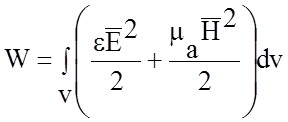 , а
, а
подинтегральное выражение плотность энергии w  :
:
![]() ;
;  ;
; 
Энергия в ЭМП распределена между электрическим и
магнитным полями и в зависимости от момента времени может находиться полностью
в электрическом поле или в магнитном поле, хотя запас энергии остается
постоянным.
Уравнение баланса для средних значений поля. На практике представляют интерес не только мгновенные
значения векторов поля, плотностей энергии, но и их среднее значение.
Усреднение происходит за отрезок времени равный периоду гармонического
колебания 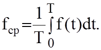
При анализе используют метод комплексных амплитуд,
который непосредственно применим в случае линейных уравнений. Обычная замена в
формуле (3.2) ![]() и
и ![]() комплексными
комплексными
векторами ![]() и
и ![]() приведет
приведет
к неправильным результатам так, как ![]() ;
; ![]() . Поэтому векторы представляют как:
. Поэтому векторы представляют как:
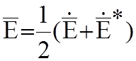 ;
; 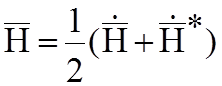 ,
,
где 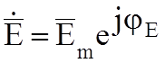 ;
; 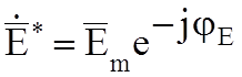 – комплексно-сопряженная амплитуда.
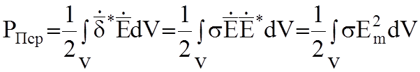
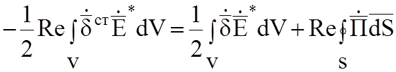
Комплексный вектор Пойнтинга и среднее
значение. Представляя вектор Пойнтинга таким образом и усредняя его за
период времени, получим:
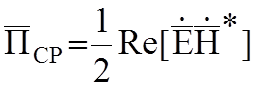 ,
,
где 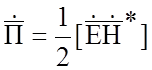 -комплексный вектор
Пойнтинга, а его вещественная часть есть среднее значение ![]() , который можно рассматривать как среднюю
, который можно рассматривать как среднюю
за период плотность потока энергии. Средний поток энергии через поверхность S,
ограничивающая объем:
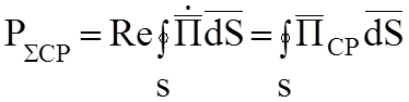
Аналогично вычисляются и другие интегралы. Выпишем
окончательные результаты.
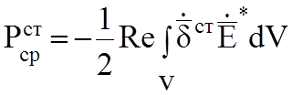
Средняя
мощность потерь  :
:
Средняя
мощность, выделяемая сторонними источниками в объем:
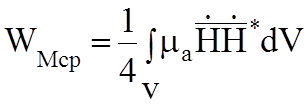
Среднее
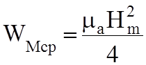
значение электрической и магнитной энергии:
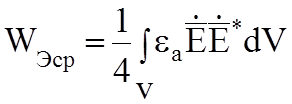 ;
; 
Среднее
значение плотностей электрической и магнитной энергии:
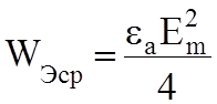 ;
; 
Среднее
за период изменение энергии равно нулю:
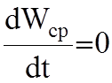
Таким
образом, усреднение по времени теоремы Умова-Пойнтинга (3.2) приводит к
уравнению:
(3.3)
В среднем за период мощность сторонних источников
расходуется на тепловые потери и на излучение из этого объема через поверхность
S. Если ![]() , то поток энергии в
, то поток энергии в
среднем выходит из объема, если ![]() , то энергия поступает
, то энергия поступает
в объем из окружающего пространства.
В электродинамике рассматривают также комплексную
мощность сторонних источников:
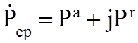
(3.4)
Вещественная
часть, или активная мощность равна средней за период мощности. Реактивная
мощность ![]() изменяется со временем по гармоническому
изменяется со временем по гармоническому
закону с частотой 2w. Это означает, что в течение периода половину времени
мощность имеет положительное значение, а вторую половину – отрицательное.
Среднее за период ![]() , то есть реактивная энергия не
, то есть реактивная энергия не
расходуется.
Резонансные
явления из уравнения баланса комплексной мощности. Выделим мнимую
часть, получим уравнение баланса реактивной мощности:
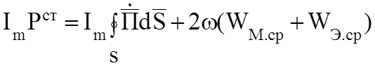 (3.5)
(3.5)
Предположим,
что объем V представляет изолированную систему. Тогда реактивный
и активный потоки энергии через поверхность S равны нулю и уравнения (3.4) и (3.3) примут вид:
 ;
; 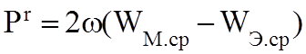 (3.6)
(3.6)
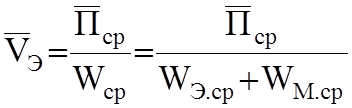
В
этом случае энергия электрического поля будет преобразовываться в магнитную и
обратно, если ![]() , то этот процесс будет протекать
, то этот процесс будет протекать
без участия сторонних источников. Реактивная мощность сторонних источников ![]() , а
, а ![]() мощность
мощность
источника будет чисто активной. Это явление называют резонансом, его условие ![]() .
.
Отношение:
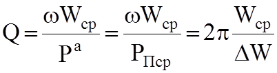 (3.7)
(3.7)
называют
добротностью изолированной системы,
где
![]() ;
; ![]() –
–
изменение энергии системы за период. Таким образом, добротность есть отношение
запаса энергии Wср и
энергии ![]() расходуемой за период Т, умноженной на 2p.
расходуемой за период Т, умноженной на 2p.
Скорость
движения энергии равна:
(3.8)
