Как найти стационарное распределение цепи маркова - Сайт, где вы сможете решить свои вопросы

В 1998 году Лоуренс Пейдж, Сергей Брин, Раджив Мотвани и Терри Виноград опубликовали статью «The PageRank Citation Ranking: Bringing Order to the Web», в которой описали знаменитый теперь алгоритм PageRank, ставший фундаментом Google. Спустя чуть менее двух десятков лет Google стал гигантом, и даже несмотря на то, что его алгоритм сильно эволюционировал, PageRank по-прежнему является «символом» алгоритмов ранжирования Google (хотя только немногие люди могут действительно сказать, какой вес он сегодня занимает в алгоритме).

С теоретической точки зрения интересно заметить, что одна из стандартных интерпретаций алгоритма PageRank основывается на простом, но фундаментальном понятии цепей Маркова. Из статьи мы увидим, что цепи Маркова — это мощные инструменты стохастического моделирования, которые могут быть полезны любому эксперту по аналитическим данным (data scientist). В частности, мы ответим на такие базовые вопросы: что такое цепи Маркова, какими хорошими свойствами они обладают, и что с их помощью можно делать?

Краткий обзор

В первом разделе мы приведём базовые определения, необходимые для понимания цепей Маркова. Во втором разделе мы рассмотрим особый случай цепей Маркова в конечном пространстве состояний. В третьем разделе мы рассмотрим некоторые из элементарных свойств цепей Маркова и проиллюстрируем эти свойства на множестве мелких примеров. Наконец, в четвёртом разделе мы свяжем цепи Маркова с алгоритмом PageRank и увидим на искусственном примере, как цепи Маркова можно применять для ранжирования узлов графа.

Примечание. Для понимания этого поста необходимы знания основ вероятностей и линейной алгебры. В частности, будут использованы следующие понятия: условная вероятность, собственный вектор и формула полной вероятности.

Что такое цепи Маркова?

Случайные переменные и случайные процессы

Прежде чем вводить понятие цепей Маркова, давайте вкратце вспомним базовые, но важные понятия теории вероятностей.

Во-первых, вне языка математики случайной величиной X считается величина, которая определяется результатом случайного явления. Его результатом может быть число (или «подобие числа», например, векторы) или что-то иное. Например, мы можем определить случайную величину как результат броска кубика (число) или же как результат бросания монетки (не число, если только мы не обозначим, например, «орёл» как 0, а «решку» как 1). Также упомянем, что пространство возможных результатов случайной величины может быть дискретным или непрерывным: например, нормальная случайная величина непрерывна, а пуассоновская случайная величина дискретна.

Далее мы можем определить случайный процесс (также называемый стохастическим) как набор случайных величин, проиндексированных множеством T, которое часто обозначает разные моменты времени (в дальнейшем мы будем считать так). Два самых распространённых случая: T может быть или множеством натуральных чисел (случайный процесс с дискретным временем), или множеством вещественных чисел (случайный процесс с непрерывным временем). Например, если мы будем бросать монетку каждый день, то зададим случайный процесс с дискретным временем, а постоянно меняющаяся стоимость опциона на бирже задаёт случайный процесс с непрерывным временем. Случайные величины в разные моменты времени могут быть независимыми друг от друга (пример с подбрасыванием монетки), или иметь некую зависимость (пример со стоимостью опциона); кроме того, они могут иметь непрерывное или дискретное пространство состояний (пространство возможных результатов в каждый момент времени).

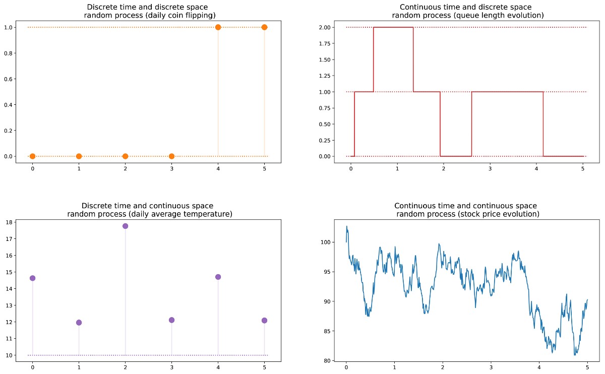
Разные виды случайных процессов (дискретные/непрерывные в пространстве/времени).

Марковское свойство и цепь Маркова

Существуют хорошо известные семейства случайных процессов: гауссовы процессы, пуассоновские процессы, авторегрессивные модели, модели скользящего среднего, цепи Маркова и другие. Каждое из этих отдельных случаев имеет определённые свойства, позволяющие нам лучше исследовать и понимать их.

Одно из свойств, сильно упрощающее исследование случайного процесса — это «марковское свойство». Если объяснять очень неформальным языком, то марковское свойство сообщает нам, что если мы знаем значение, полученное каким-то случайным процессом в заданный момент времени, то не получим никакой дополнительной информации о будущем поведении процесса, собирая другие сведения о его прошлом. Более математическим языком: в любой момент времени условное распределение будущих состояний процесса с заданными текущим и прошлыми состояниями зависит только от текущего состояния, но не от прошлых состояний (свойство отсутствия памяти). Случайный процесс с марковским свойством называется марковским процессом.

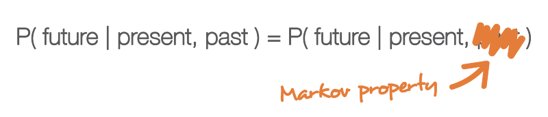
Марковское свойство обозначает, что если мы знаем текущее состояние в заданный момент времени, то нам не нужна никакая дополнительная информация о будущем, собираемая из прошлого.

На основании этого определения мы можем сформулировать определение «однородных цепей Маркова с дискретным временем» (в дальнейшем для простоты мы их будем называть «цепями Маркова»). Цепь Маркова — это марковский процесс с дискретным временем и дискретным пространством состояний. Итак, цепь Маркова — это дискретная последовательность состояний, каждое из которых берётся из дискретного пространства состояний (конечного или бесконечного), удовлетворяющее марковскому свойству.

Математически мы можем обозначить цепь Маркова так:

где в каждый момент времени процесс берёт свои значения из дискретного множества E, такого, что

Тогда марковское свойство подразумевает, что у нас есть

Снова обратите внимание, что эта последняя формула отражает тот факт, что для хронологии (где я нахожусь сейчас и где я был раньше) распределение вероятностей следующего состояния (где я буду дальше) зависит от текущего состояния, но не от прошлых состояний.

Примечание. В этом ознакомительном посте мы решили рассказать только о простых однородных цепях Маркова с дискретным временем. Однако существуют также неоднородные (зависящие от времени) цепи Маркова и/или цепи с непрерывным временем. В этой статье мы не будем рассматривать такие вариации модели. Стоит также заметить, что данное выше определение марковского свойства чрезвычайно упрощено: в истинном математическом определении используется понятие фильтрации, которое выходит далеко за пределы нашего вводного знакомства с моделью.

Характеризуем динамику случайности цепи Маркова

В предыдущем подразделе мы познакомились с общей структурой, соответствующей любой цепи Маркова. Давайте посмотрим, что нам нужно, чтобы задать конкретный «экземпляр» такого случайного процесса.

Сначала заметим, что полное определение характеристик случайного процесса с дискретным временем, не удовлетворяющего марковскому свойству, может быть сложным занятием: распределение вероятностей в заданный момент времени может зависеть от одного или нескольких моментов в прошлом и/или будущем. Все эти возможные временные зависимости потенциально могут усложнить создание определения процесса.

Однако благодаря марковскому свойству динамику цепи Маркова определить довольно просто. И в самом деле. нам нужно определить только два аспекта: исходное распределение вероятностей (то есть распределение вероятностей в момент времени n=0), обозначаемое

и матрицу переходных вероятностей (которая даёт нам вероятности того, что состояние в момент времени n+1 является последующим для другого состояния в момент n для любой пары состояний), обозначаемую

Если два этих аспекта известны, то полная (вероятностная) динамика процесса чётко определена. И в самом деле, вероятность любого результата процесса тогда можно вычислить циклически.

Пример: допустим, мы хотим знать вероятность того, что первые 3 состояния процесса будут иметь значения (s0, s1, s2). То есть мы хотим вычислить вероятность

Здесь мы применяем формулу полной вероятности, гласящую, что вероятность получения (s0, s1, s2) равна вероятности получения первого s0, умноженного на вероятность получения s1 с учётом того, что ранее мы получили s0, умноженного на вероятность получения s2 с учётом того, что мы получили ранее по порядку s0 и s1. Математически это можно записать как

И затем проявляется упрощение, определяемое марковским допущением. И в самом деле, в случае длинных цепей мы получим для последних состояний сильно условные вероятности. Однако в случае цепей Маркова мы можем упростить это выражение, воспользовавшись тем, что

получив таким образом

Так как они полностью характеризуют вероятностную динамику процесса, многие сложные события можно вычислить только на основании исходного распределения вероятностей q0 и матрицы переходной вероятности p. Стоит также привести ещё одну базовую связь: выражение распределения вероятностей во время n+1, выраженное относительно распределения вероятностей во время n

Цепи Маркова в конечных пространствах состояний

Представление в виде матриц и графов

Здесь мы допустим, что во множестве E есть конечное количество возможных состояний N:

Тогда исходное распределение вероятностей можно описать как вектор-строку q0 размером N, а переходные вероятности можно описать как матрицу p размером N на N, такую что

Преимущество такой записи заключается в том, что если мы обозначим распределение вероятностей на шаге n вектором-строкой qn, таким что его компоненты задаются

тогда простые матричные связи при этом сохраняются

(здесь мы не будем рассматривать доказательство, но воспроизвести его очень просто).

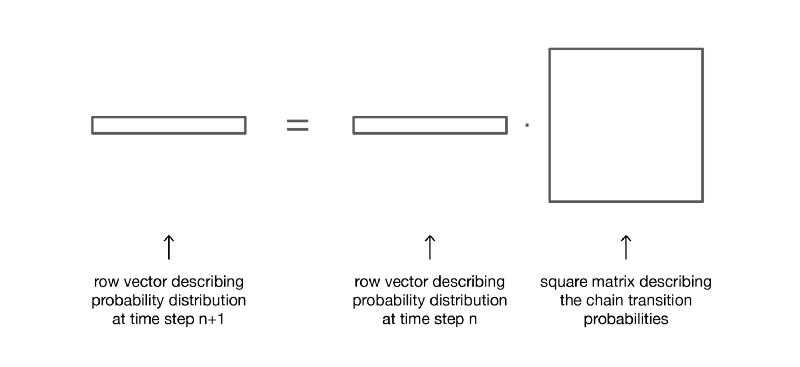
Если умножить справа вектор-строку, описывающий распределение вероятностей на заданном этапе времени, на матрицу переходных вероятностей, то мы получим распределение вероятностей на следующем этапе времени.

Итак, как мы видим, переход распределения вероятностей из заданного этапа в последующий определяется просто как умножение справа вектора-строки вероятностей исходного шага на матрицу p. Кроме того, это подразумевает, что у нас есть

Динамику случайности цепи Маркова в конечном пространстве состояний можно с лёгкостью представить как нормированный ориентированный граф, такой что каждый узел графа является состоянием, а для каждой пары состояний (ei, ej) существует ребро, идущее от ei к ej, если p(ei,ej)>0. Тогда значение ребра будет той же вероятностью p(ei,ej).

Пример: читатель нашего сайта

Давайте проиллюстрируем всё это простым примером. Рассмотрим повседневное поведение вымышленного посетителя сайта. В каждый день у него есть 3 возможных состояния: читатель не посещает сайт в этот день (N), читатель посещает сайт, но не читает пост целиком (V) и читатель посещает сайт и читает один пост целиком (R ). Итак, у нас есть следующее пространство состояний:

Допустим, в первый день этот читатель имеет вероятность 50% только зайти на сайт и вероятность 50% посетить сайт и прочитать хотя бы одну статью. Вектор, описывающий исходное распределение вероятностей (n=0) тогда выглядит так:

Также представим, что наблюдаются следующие вероятности:

когда читатель не посещает один день, то имеет вероятность 25% не посетить его и на следующий день, вероятность 50% только посетить его и 25% — посетить и прочитать статью
когда читатель посещает сайт один день, но не читает, то имеет вероятность 50% снова посетить его на следующий день и не прочитать статью, и вероятность 50% посетить и прочитать
когда читатель посещает и читает статью в один день, то имеет вероятность 33% не зайти на следующий день (надеюсь, этот пост не даст такого эффекта!), вероятность 33% только зайти на сайт и 34% — посетить и снова прочитать статью

Тогда у нас есть следующая переходная матрица:

Из предыдущего подраздела мы знаем как вычислить для этого читателя вероятность каждого состояния на следующий день (n=1)

Вероятностную динамику этой цепи Маркова можно графически представить так:

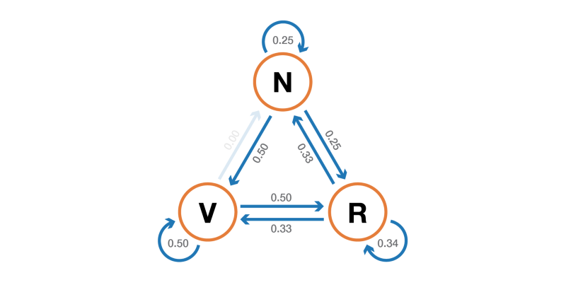
Представление в виде графа цепи Маркова, моделирующей поведение нашего придуманного посетителя сайта.

Свойства цепей Маркова

В этом разделе мы расскажем только о некоторых самых базовых свойствах или характеристиках цепей Маркова. Мы не будем вдаваться в математические подробности, а представим краткий обзор интересных моментов, которые необходимо изучить для использования цепей Маркова. Как мы видели, в случае конечного пространства состояний цепь Маркова можно представить в виде графа. В дальнейшем мы будем использовать графическое представление для объяснения некоторых свойств. Однако не стоит забывать, что эти свойства необязательно ограничены случаем конечного пространства состояний.

Разложимость, периодичность, невозвратность и возвратность

В этом подразделе давайте начнём с нескольких классических способов характеризации состояния или целой цепи Маркова.

Во-первых, мы упомянем, что цепь Маркова неразложима, если можно достичь любого состояния из любого другого состояния (необязательно, что за один шаг времени). Если пространство состояний конечно и цепь можно представить в виде графа, то мы можем сказать, что граф неразложимой цепи Маркова сильно связный (теория графов).

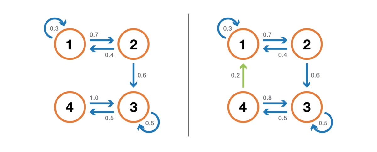
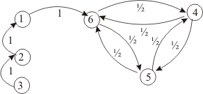
Иллюстрация свойства неразложимости (несокращаемости). Цепь слева нельзя сократить: из 3 или 4 мы не можем попасть в 1 или 2. Цепь справа (добавлено одно ребро) можно сократить: каждого состояния можно достичь из любого другого.

Состояние имеет период k, если при уходе из него для любого возврата в это состояние нужно количество этапов времени, кратное k (k — наибольший общий делитель всех возможных длин путей возврата). Если k = 1, то говорят, что состояние является апериодическим, а вся цепь Маркова является апериодической, если апериодичны все её состояния. В случае неприводимой цепи Маркова можно также упомянуть, что если одно состояние апериодическое, то и все другие тоже являются апериодическими.

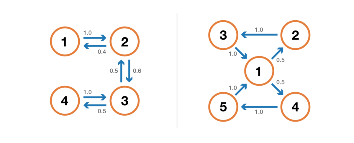
Иллюстрация свойства периодичности. Цепь слева периодична с k=2: при уходе из любого состояния для возврата в него всегда требуется количество шагов, кратное 2. Цепь справа имеет период 3.

Состояние является невозвратным, если при уходе из состояния существует ненулевая вероятность того, что мы никогда в него не вернёмся. И наоборот, состояние считается возвратным, если мы знаем, что после ухода из состояния можем в будущем вернуться в него с вероятностью 1 (если оно не является невозвратным).

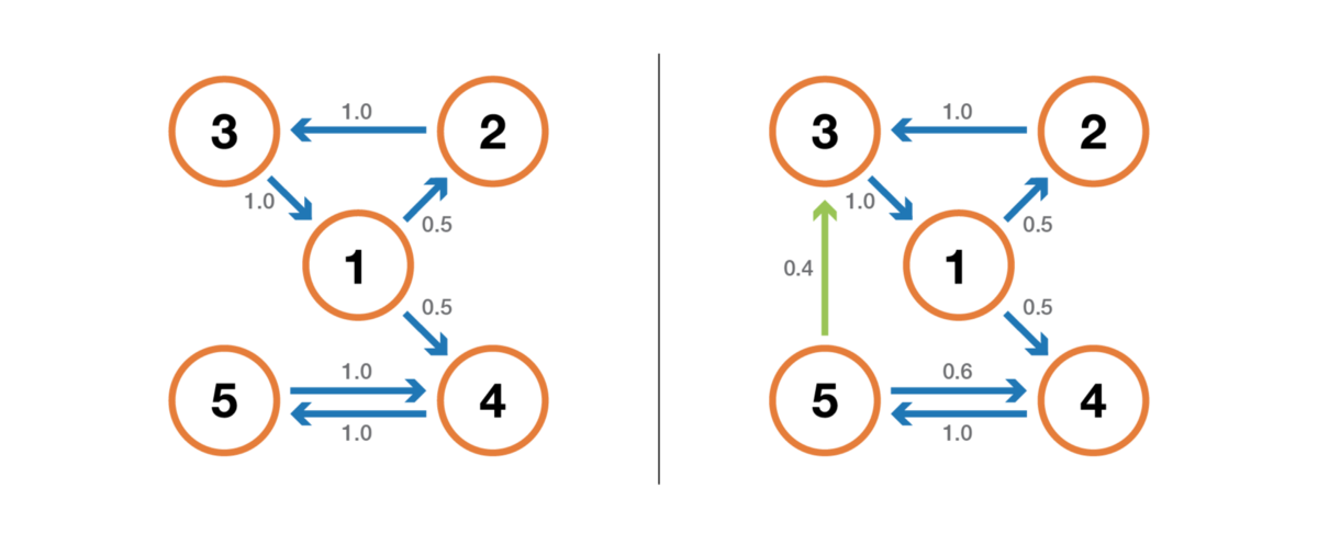
Иллюстрация свойства возвратности/невозвратности. Цепь слева имеет такие свойства: 1, 2 и 3 невозвратны (при уходе из этих точек мы не можем быть абсолютно уверены, что вернёмся в них) и имеют период 3, а 4 и 5 возвратны (при уходе из этих точек мы абсолютно уверены, что когда-нибудь к ним вернёмся) и имеют период 2. Цепь справа имеет ещё одно ребро, делающее всю цепь возвратной и апериодической.

Для возвратного состояния мы можем вычислить среднее время возвратности, которое является ожидаемым временем возврата при покидании состояния. Заметьте, что даже вероятность возврата равна 1, то это не значит, что ожидаемое время возврата конечно. Поэтому среди всех возвратных состояний мы можем различать положительные возвратные состояния (с конечным ожидаемым временем возврата) и нулевые возвратные состояния (с бесконечным ожидаемым временем возврата).

Стационарное распределение, предельное поведение и эргодичность

В этом подразделе мы рассмотрим свойства, характеризующие некоторые аспекты (случайной) динамики, описываемой цепью Маркова.

Распределение вероятностей π по пространству состояний E называют стационарным распределением, если оно удовлетворяет выражению

Так как у нас есть

Тогда стационарное распределение удовлетворяет выражению

По определению, стационарное распределение вероятностей со временем не изменяется. То есть если исходное распределение q является стационарным, тогда оно будет одинаковых на всех последующих этапах времени. Если пространство состояний конечно, то p можно представить в виде матрицы, а π — в виде вектора-строки, и тогда мы получим

Это снова выражает тот факт, что стационарное распределение вероятностей со временем не меняется (как мы видим, умножение справа распределения вероятностей на p позволяет вычислить распределение вероятностей на следующем этапе времени). Учтите, что неразложимая цепь Маркова имеет стационарное распределение вероятностей тогда и только тогда, когда одно из её состояний является положительным возвратным.

Ещё одно интересное свойство, связанное с стационарным распределением вероятностей, заключается в следующем. Если цепь является положительной возвратной (то есть в ней существует стационарное распределение) и апериодической, тогда, какими бы ни были исходные вероятности, распределение вероятностей цепи сходится при стремлении интервалов времени к бесконечности: говорят, что цепь имеет предельное распределение, что является ничем иным, как стационарным распределением. В общем случае его можно записать так:

Ещё раз подчеркнём тот факт, что мы не делаем никаких допущений об исходном распределении вероятностей: распределение вероятностей цепи сводится к стационарному распределению (равновесному распределению цепи) вне зависимости от исходных параметров.

Наконец, эргодичность — это ещё одно интересное свойство, связанное с поведением цепи Маркова. Если цепь Маркова неразложима, то также говорится, что она «эргодическая», потому что удовлетворяет следующей эргодической теореме. Допустим, у нас есть функция f(.), идущая от пространства состояний E к оси (это может быть, например, цена нахождения в каждом состоянии). Мы можем определить среднее значение, перемещающее эту функцию вдоль заданной траектории (временное среднее). Для n-ных первых членов это обозначается как

Также мы можем вычислить среднее значение функции f на множестве E, взвешенное по стационарному распределению (пространственное среднее), которое обозначается

Тогда эргодическая теорема говорит нам, что когда траектория становится бесконечно длинной, временное среднее равно пространственному среднему (взвешенному по стационарному распределению). Свойство эргодичности можно записать так:

Иными словами, оно обозначает, что в пределе ранее поведение траектории становится несущественным и при вычислении временного среднего важно только долговременное стационарное поведение.

Вернёмся к примеру с читателем сайта

Снова рассмотрим пример с читателем сайта. В этом простом примере очевидно, что цепь неразложима, апериодична и все её состояния положительно возвратны.

Чтобы показать, какие интересные результаты можно вычислить с помощью цепей Маркова, мы рассмотрим среднее время возвратности в состояние R (состояние «посещает сайт и читает статью»). Другими словами, мы хотим ответить на следующий вопрос: если наш читатель в один день заходит на сайт и читает статью, то сколько дней нам придётся ждать в среднем того, что он снова зайдёт и прочитает статью? Давайте попробуем получить интуитивное понятие о том, как вычисляется это значение.

Сначала мы обозначим

Итак, мы хотим вычислить m(R,R). Рассуждая о первом интервале, достигнутом после выхода из R, мы получим

Однако это выражение требует, чтобы для вычисления m(R,R) мы знали m(N,R) и m(V,R). Эти две величины можно выразить аналогичным образом:

Итак, у нас получилось 3 уравнения с 3 неизвестными и после их решения мы получим m(N,R) = 2.67, m(V,R) = 2.00 и m(R,R) = 2.54. Значение среднего времени возвращения в состояние R тогда равно 2.54. То есть с помощью линейной алгебры нам удалось вычислить среднее время возвращения в состояние R (а также среднее время перехода из N в R и среднее время перехода из V в R).

Чтобы закончить с этим примером, давайте посмотрим, каким будет стационарное распределение цепи Маркова. Чтобы определить стационарное распределение, нам нужно решить следующее уравнение линейной алгебры:

То есть нам нужно найти левый собственный вектор p, связанный с собственным вектором 1. Решая эту задачу, мы получаем следующее стационарное распределение:

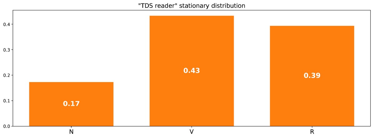
Стационарное распределение в примере с читателем сайта.

Можно также заметить, что π( R ) = 1/m(R,R), и если немного поразмыслить, то это тождество довольно логично (но подробно об этом мы говорить не будем).

Поскольку цепь неразложима и апериодична, это означает, что в длительной перспективе распределение вероятностей сойдётся к стационарному распределению (для любых исходных параметров). Иными словами, каким бы ни было исходное состояние читателя сайта, если мы подождём достаточно долго и случайным образом выберем день, то получим вероятность π(N) того, что читатель не зайдёт на сайт в этот день, вероятность π(V) того, что читатель зайдёт, но не прочитает статью, и вероятность π® того, что читатель зайдёт и прочитает статью. Чтобы лучше уяснить свойство сходимости, давайте взглянем на следующий график, показывающий эволюцию распределений вероятностей, начинающихся с разных исходных точек и (быстро) сходящихся к стационарному распределению:

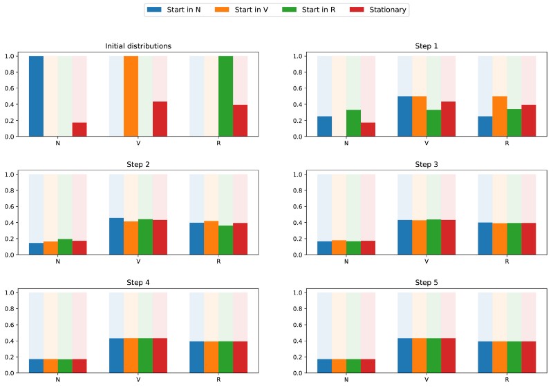
Визуализация сходимости 3 распределений вероятностей с разными исходными параметрами (синяя, оранжевая и зелёная) к стационарному распределению (красная).

Классический пример: алгоритм PageRank

Настало время вернуться к PageRank! Но прежде чем двигаться дальше, стоит упомянуть, что интерпретация PageRank, данная в этой статье, не единственно возможная, и авторы оригинальной статьи при разработке методики не обязательно рассчитывали на применение цепей Маркова. Однако наша интерпретация хороша тем, что очень понятна.

Произвольный веб-пользователь

PageRank пытается решить следующую задачу: как нам ранжировать имеющееся множество (мы можем допустить, что это множество уже отфильтровано, например, по какому-то запросу) с помощью уже существующих между страницами ссылок?

Чтобы решить эту задачу и иметь возможность отранжировать страницы, PageRank приблизительно выполняет следующий процесс. Мы считаем, что произвольный пользователь Интернета в исходный момент времени находится на одной из страниц. Затем этот пользователь начинает случайным образом начинает перемещаться, щёлкая на каждой странице по одной из ссылок, которые ведут на другую страницу рассматриваемого множества (предполагается, что все ссылки, ведущие вне этих страниц, запрещены). На любой странице все допустимые ссылки имеют одинаковую вероятность нажатия.

Так мы задаём цепь Маркова: страницы — это возможные состояния, переходные вероятности задаются ссылками со страницы на страницу (взвешенными таким образом, что на каждой странице все связанные страницы имеют одинаковую вероятность выбора), а свойства отсутствия памяти чётко определяются поведением пользователя. Если также предположить, что заданная цепь положительно возвратная и апериодичная (для удовлетворения этим требованиям применяются небольшие хитрости), тогда в длительной перспективе распределение вероятностей «текущей страницы» сходится к стационарному распределению. То есть какой бы ни была начальная страница, спустя длительное время каждая страница имеет вероятность (почти фиксированную) стать текущей, если мы выбираем случайный момент времени.

В основе PageRank лежит такая гипотеза: наиболее вероятные страницы в стационарном распределении должны быть также и самыми важными (мы посещаем эти страницы часто, потому что они получают ссылки со страниц, которые в процессе переходов тоже часто посещаются). Тогда стационарное распределение вероятностей определяет для каждого состояния значение PageRank.

Искусственный пример

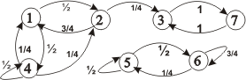
Чтобы это стало намного понятнее, давайте рассмотрим искусственный пример. Предположим, что у нас есть крошечный веб-сайт с 7 страницами, помеченными от 1 до 7, а ссылки между этими страницами соответствуют следующему графу.

Ради понятности вероятности каждого перехода в показанной выше анимации не показаны. Однако поскольку подразумевается, что «навигация» должна быть исключительно случайной (это называют «случайным блужданием»), то значения можно легко воспроизвести из следующего простого правила: для узла с K исходящими ссылками (странице с K ссылками на другие страницы) вероятность каждой исходящей ссылки равна 1/K. То есть переходная матрица вероятностей имеет вид:

где значения 0.0 заменены для удобства на “.”. Прежде чем выполнять дальнейшие вычисления, мы можем заметить, что эта цепь Маркова является неразложимой и апериодической, то есть в длительной перспективе система сходится к стационарному распределению. Как мы видели, можно вычислить это стационарное распределение, решив следующую левую задачу собственного вектора

Сделав так, мы получим следующие значения PageRank (значения стационарного распределения) для каждой страницы

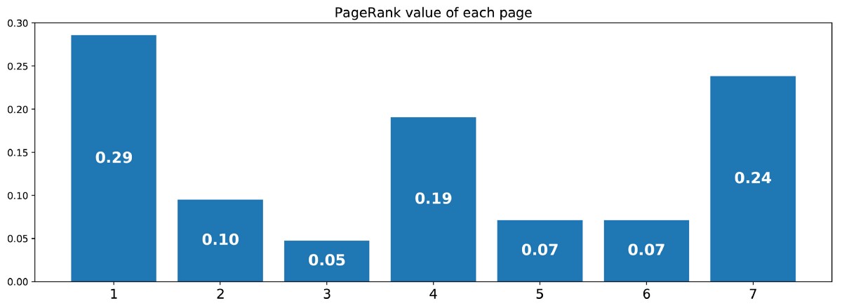
Значения PageRank, вычисленные для нашего искусственного примера из 7 страниц.

Тогда ранжирование PageRank этого крошечного веб-сайта имеет вид 1 > 7 > 4 > 2 > 5 = 6 > 3.

Выводы

Основные выводы из этой статьи:

случайные процессы — это наборы случайных величин, часто индексируемые по времени (индексы часто обозначают дискретное или непрерывное время)
для случайного процесса марковское свойство означает, что при заданном текущем вероятность будущего не зависит от прошлого (это свойство также называется «отсутствием памяти»)
цепь Маркова с дискретным временем — это случайные процессы с индексами дискретного времени, удовлетворяющие марковскому свойству
марковское свойство цепей Маркова сильно облегчает изучение этих процессов и позволяет вывести различные интересные явные результаты (среднее время возвратности, стационарное распределение…)
одна из возможных интерпретаций PageRank (не единственная) заключается в имитации веб-пользователя, случайным образом перемещающегося от страницы к странице; при этом показателем ранжирования становится индуцированное стационарное распределение страниц (грубо говоря, на самые посещаемые страницы в устоявшемся состоянии должны ссылаться другие часто посещаемые страницы, а значит, самые посещаемые должны быть наиболее релевантными)

В заключение ещё раз подчеркнём, насколько мощным инструментом являются цепи Маркова при моделировании задач, связанных со случайной динамикой. Благодаря их хорошим свойствам они используются в различных областях, например, в теории очередей (оптимизации производительности телекоммуникационных сетей, в которых сообщения часто должны конкурировать за ограниченные ресурсы и ставятся в очередь, когда все ресурсы уже заняты), в статистике (хорошо известные методы Монте-Карло по схеме цепи Маркова для генерации случайных переменных основаны на цепях Маркова), в биологии (моделирование эволюции биологических популяций), в информатике (скрытые марковские модели являются важными инструментами в теории информации и распознавании речи), а также в других сферах.

Разумеется, огромные возможности, предоставляемые цепями Маркова с точки зрения моделирования и вычислений, намного шире, чем рассмотренные в этом скромном обзоре. Поэтому мы надеемся, что нам удалось пробудить у читателя интерес к дальнейшему изучению этих инструментов, которые занимают важное место в арсенале учёного и эксперта по данным.

Источник

Эргодические теоремы для цепей Маркова

Теорема (основная
эргодическая теорема). Рассмотрим
неразложимую, непериодическую, возвратную
цепь Маркова со счётным числом состояний,
тогда имеет место равенство

При этих же условиях

.

Теорема. Для
неразложимой, непериодической, возвратной
и положительной цепи Маркова со счётным
числом состояний существуют пределы

,
где

и однозначно определяются условиями:

–уравнение Колмогорова для финальных
вероятностей,

–условием нормировки для финальных
вероятностей.

Распределение
вероятностей _i
называется финальным или эргодическим,
а цепь Маркова называется эргодической.

Теорема (альтернативы).
Пусть для марковской цепи со счётным
числом состояний существуют пределы

,
при этом выполняется равенство

,
тогда возможна одна из двух альтернатив:
все _i=0
или

.

Если

,
то набор вероятностей _i
образует единственное
стационарное распределение вероятностей
состояний цепи Маркова.

Если _i=0,
то не существует
стационарного распределения для
рассматриваемой цепи Маркова.

Теорема (эргодическая
теорема для цепей Маркова с конечным
числом состояний). Для неразложимой
непериодической цепи Маркова с конечным
числом состояний существуют пределы

не зависящие от j и
удовлетворяющие условию нормировки.

Таким образом, если
цепь Маркова неразложимая, непериодическая,
возвратная и положительная, то для неё
существует стационарное (финальное)
распределение вероятностей.

Определение. Если
для однородной цепи Маркова существуют
финальные вероятности, то говорят, что
для этой цепи существует стационарный
режим функционирования.

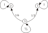
Пример
2.6. Найти финальные вероятности для
цепи Маркова заданной графом

Решение:
Данная цепь Маркова является неразложимой
и апериодической, так как d(1)=d(2)=1.
Кроме того, она имеет конечное число
состояний, поэтому является эргодической.

Матрица
вероятностей переходов

.

Составим
систему уравнений для нахождения
финальных вероятностей:

откуда находим
₁=10/17, ₂=7/17.

Вероятностно-временные характеристики цепи Маркова

Распределение
вероятностей состояний цепи Маркова
является наиболее важной её характеристикой.
Но также представляют интерес и некоторые
другие её характеристики.

Вероятность перехода
из несущественного состояния в замкнутый
класс.

Обозначим _i(S_k)
вероятность перехода цепи Маркова из
несущественного состояния i
в замкнутый класс S_k,
p_ij
– вероятности перехода из i-го
состояния в j-ое. Тогда
_i(S_k)
является решением неоднородной системой
линейных алгебраических уравнений
следующего вида.

где T – множество
несущественных состояний.

Среднее время перехода
из несущественного состояния в замкнутый
класс.

Пусть для цепи Маркова
единственный замкнутый класс S.
Обозначим m_i(S)
– среднее значение времени перехода
цепи Маркова из несущественного состояния
i в замкнутый класс
S. Учитывая, что если
из состояния i можно
сразу попасть в класс S_k,
то время перехода равно единице, а если
этот переход выполняется в несущественное
состояние j, тогда
суммарное время перехода составляет
1+ m_j(S),
где первое слагаемое, равное единице,
определяет первый шаг, а второе: m_j(S)
– среднее значение времени перехода
из состояния j в класс
S.

В силу формулы полной
вероятности для условных математических
ожиданий, можно записать систему линейных
неоднородных уравнений для определения
m_i(S):

Пример
2.7. Студент может перейти на следующий
курс с вероятностью p, с
вероятностью q может
остаться на повторное обучение, а с
вероятностью r может быть
отчислен (p+q+r=1).
Восстановление невозможно, но с
вероятностью pможно вновь
поступить на первый курс. Записать
матрицу вероятностей переходов за один
шаг и найти среднее время перехода в
эргодическое множество.

Решение:
Будем считать, что образование занимает
5 лет, тогда состояния S₁,
S₂, S₃,
S₄, S₅
– соответствуют обучению с первого
по пятый курс, S₀,
– абитуриент, S₆
– специалист. По определению S₀,
S₁, S₂,
S₃, S₄,
S₅ – несущественные
состояния, S₆ –
эргодическое множество из одного
состояния.

Тогда матрица
переходов за один шаг в каноническом
виде может быть записана

Через m_i
обозначим среднее время перехода из
несущественного состояния S_i,

в эргодическое состояние S₆.
Тогда можно записать систему уравнений:

Будем решать
систему методом Крамера. Найдем
определитель системы:

Найдем _i:

Следовательно,

.

Аналогично
находим для остальных состояний, и
записываем ответ в общем виде.

Ответ:

,

.

Если цепь Маркова
содержит k замкнутых
классов, то для нахождения среднего
времени перехода из несущественного
состояния в k-ый
замкнутый класс S_k,
необходимо учитывать вероятность
перехода в этот замкнутый класс, то есть
находить условное время перехода
m_i(S_k/H_k),
где H_k
– событие, состоящее в том, что из i-го
состояния мы перешли в k-ый
замкнутый класс. Это время перехода
определяется равенством:

где m_i(S_k/H_k)
определяется аналогично m_i(S)
для цепи Маркова с единственным замкнутым
классом состояний.

Пример
2.8. Найдите вероятность и условное
среднее время перехода из несущественного
состояния в замкнутый класс для цепи
Маркова, заданных матрицей переходов
за один шаг систем

Решение:
Граф состояний для заданной цепи Маркова
имеет вид

Очевидно, что
у рассматриваемой цепи состояние 3 –
несущественное и есть два неразложимых
класса S₁=1,
S₂=2.

Следовательно,
рассмотри две гипотезы:

H₁
– произошел переход в замкнутый S₁;

H₂
– произошел переход в замкнутый S₂.

Тогда условное
среднее время перехода из несущественного
состояния в замкнутые классы S₁
и S₂ определяется
по формулам:

где ₃(H_i)
– вероятность события H_i,
то есть вероятность перехода из
несущественного состояния 3 в i-ый
замкнутый класс.

Вероятности
перехода из несущественного состояния
3 в замкнутые классы S₁
и S₂ определяем
по формулам

Откуда
получаем:
,
.

Для m₃(S₁,H₁)
и m₃(S₂,H₂)
имеем систему уравнений:

,

;

,

.

Тогда условное
среднее время перехода из несущественного
состояния в замкнутые классы

составляет:

Среднее время перехода
из состояния в состояние внутри замкнутого
класса

Рассмотрим некоторый
замкнутый класс S.
Обозначим m_ij
– среднее значение времени перехода
из состояния i в
состояние j внутри
замкнутого класса для  i, j S.

Тогда можно получить
систему линейных неоднородных
алгебраических уравнений, определяющих
значения m_ij:

Из полученной системы
можно найти следующие соотношения:

,

, (2.4)

из которых следует, что среднее время
возвращения в возвратное состояние j
обратно пропорционально финальной
вероятности этого состояния, поэтому
для положительных состояний оно конечно,
а для нулевых – бесконечно.

Распределение
вероятностей времени пребывания в j-м
состоянии

Обозначим _j
– время (число тактов) пребывания системы
в состоянии j. Достаточно
очевидны следующие равенства

то есть время пребывания системы в любом
состоянии имеет геометрическое
распределение с параметром равным p_jj
– вероятности остаться в этом состоянии
на следующем шаге.

Среднее значение
времени пребывания в j-м
состоянии составляет

Статистический смысл
стационарных (финальных) вероятностей

Обозначим T_j
– среднее число шагов от момента выхода
из j-го состояния до
момента возвращения цепи Маркова в это
состояние, тогда по формуле полной
вероятности можно записать

тогда, равенство (2.4) перепишем следующим
образом

Здесь числитель равен
среднему значению времени, проведённому
системой в j-ом
состоянии, а знаменатель равен сумме
этого значения и среднему значению
длины интервала от момента выхода цепи
из j-го состояния до
момента возвращения в него. Следовательно,
стационарные (финальные) вероятности
для цепи Маркова можно интерпретировать
как среднее значение доли времени,
проведённого цепью в j-ом
состоянии.

Задачи для самостоятельного решения

Построить
граф состояний следующего случайного
процесса: устройство S
состоит из двух узлов, каждый из которых
в случайный момент времени может выйти
их строя, после чего мгновенно начинается
ремонт узла, продолжающийся случайное
время.
На окружности
отмечено 5 точек. Процесс попадает из
любой данной точки в одну из соседних
с вероятностью 0,5. Записать матрицу
переходов за один шаг. Найти матрицу
переходов за 2,3 шага.
В учениях
участвуют два корабля, которые
одновременно производят выстрелы друг
в друга через равные промежутки времени.
При каждом выстреле корабль А поражает
корабль Б с вероятностью 1/2, а корабль
Б поражает корабль А с вероятностью
3/8. Предполагается, что при любом
попадании корабль выходит из строя.
Рассматриваются результаты серии
выстрелов. Найти матрицу перехода, если
состояниями цепи являются комбинации
кораблей, оставшихся в строю: Е₁
– оба корабля в строю, Е₂ – в строю
только корабль А, Е₃ – в строю
только корабль Б, Е₄ – оба корабля
поражены.
В сказочной
стране Оз никогда не бывает двух
солнечных дней подряд. Если сегодня
ясно, то завтра будет плохая погода –
снег или дождь с равной вероятностью.
Если сегодня дождь, то завтра погода
изменится с вероятностью 0,5. Если она
изменится, то в половине случаев будет
ясно. Записать матрицу переходов за
один шаг. Найти вероятность того, что
послезавтра будет ясно, если сегодня
ясно.
N-черных
и N-белых шаров
размещены по двум урнам так, что в каждой
из них по N шаров.
Число черных шаров первой урны определяет
состояние системы. На каждом шаге
случайно выбираются по одному шару из
каждой урны и меняются местами. Записать
матрицу вероятностей переходов за один
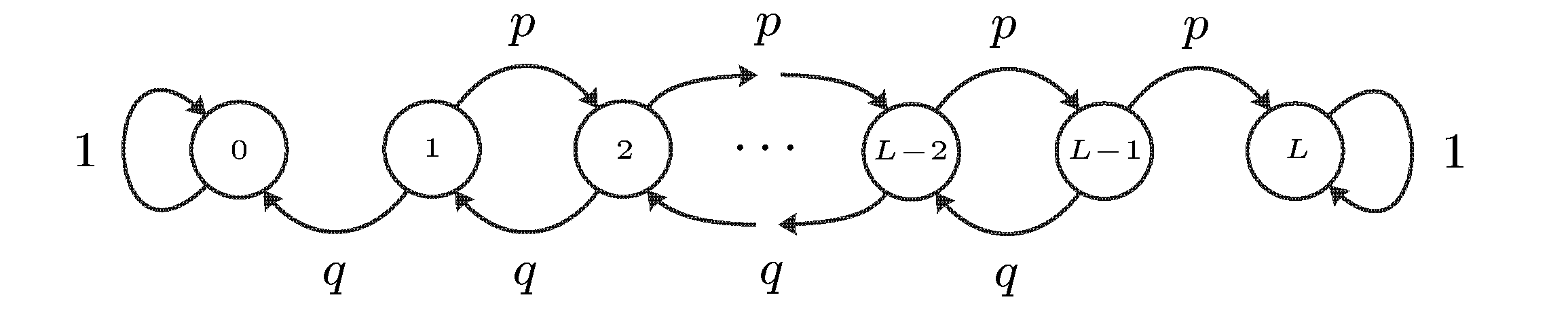
шаг. И найти финальные вероятности.
Пусть целые
числа M>0 и N>0 (M+N=L) –
начальные капиталы соответственно
первого и второго игроков. Проводятся
последовательно игры, в результате
каждой из которых с вероятностью

капитал первого игрока увеличивается
на 1 и с вероятностью q=1–p капитал
первого игрока уменьшается на 1.
Результаты любой игры не зависят от
результатов любых других игр. Пусть S_n
– капитал первого игрока после n
игр. Предполагается, что в случае S_n=0
или S_n=N+M игра
прекращается (ситуация разорения одного
игрока). Построить стохастический граф
цепи, провести классификацию состояний
и найти переходную матрицу. Найти
вероятность разорения первого игрока.
Рассмотреть случай, когда один из
игроков бесконечно богат. Указание:
граф переходов имеет вид:

Через
фиксированные промежутки времени
проводится контроль технического
состояния банкомата, который может
находиться в одном из трех состояний:
S₁ – работает, S₂ –
не работает и ожидает ремонта, S₃
– ремонтируется. Предполагается, что
процесс, характеризующий состояние
прибора является однородной цепью
Маркова с переходной матрицей

Найти
неизвестные элементы матрицы P и
вычислить P(2) при условии, что в
начальный момент времени банкомат был
исправен. Найти среднее время перехода
внутри замкнутого класса.

Классифицировать
состояния для марковской цепи, заданной
матрицей вероятностей переходов P₁,
записать ее в каноническом виде и найти
среднее время перехода из одного
состояния в другое внутри замкнутого
класса (все возможные варианты).

;
;

;
.

Две автомашины
A и B сдаются в аренду по одной и той же
цене. Каждая из них может находиться в
одном из двух состояний: i₁
– машина работает хорошо, i₂
– машина требует ремонта, которые
образуют цепь Маркова. Матрицы
вероятностей переходов между состояниями
за сутки для этих машин равны
соответственно:

Определить
финальные вероятности состояний для
обеих автомашин. Какую автомашину стоит
арендовать?

Цепь Маркова
задана графом (рис.4). Найти стационарное
распределение вероятностей, если оно
существует.

Рис.
4.

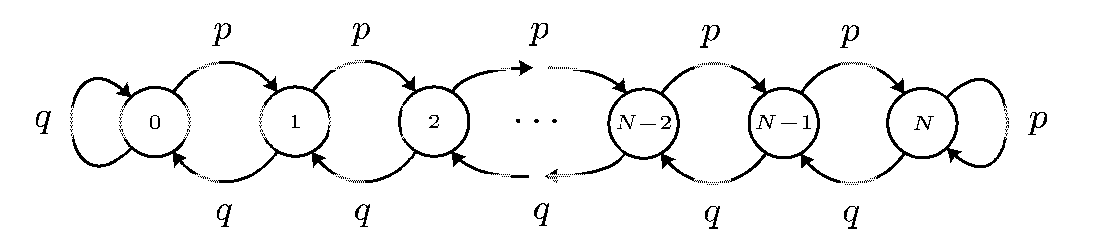
Цепь Маркова
имеет множество допустимых состояний
E=0,1,2,…,N
и описывается графом (рис.5), где 0<p<1,
q=1–p. Доказать, что цепь является
эргодической, и найти стационарное
распределение вероятностей.

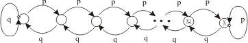
Рис.
5.

Провести
классификации состояний и записать
матрицы переходов в каноническом виде
для следующих цепей Маркова

a)

; б)

;

в)

; г)

;

е)

,

.

Цепь Маркова
имеет множество состояний -6,-5,…,0,1,…,6.
Переходные вероятности определяются
соотношениями

Провести
классификацию состояний цепи Маркова
и множества ее состояний, если выполняются
равенства:

а)

;

б)

;

в)

.

Цепь Маркова
задана матрицей переходов за один шаг.
Найдите финальные вероятности состояний
цепи Маркова.

a)

; б)

;

в)

; г)

Найдите
вероятность и условное, при условии
попадания в S_k,
среднее время перехода из несущественного
состояния в замкнутый класс для цепи
Маркова, заданных матрицей вероятностей
переходов за один шаг.

; в)

;

б)

; г)

.

Найдите
вероятность и среднее время перехода
из несущественного состояния в замкнутый
класс для цепи Маркова, заданных графом
вероятностей переходов за один шаг:

Найдите
среднее время перехода внутри замкнутого
класса.

Найдите
вероятность и условное среднее время
перехода из несущественного состояния
в замкнутый класс для цепи Маркова,
заданных графом вероятностей переходов
за один шаг:

Найдите среднее
время перехода внутри замкнутых классов.

В процессе
эксплуатации ЭВМ может рассматриваться
как физическая система, которая в
результате проверки может оказаться
в одном из следующих состояний: x₁
– ЭВМ полностью исправна; x₂
– ЭВМ имеет незначительные неисправности
в ОП, но может решать задачи; x₃
– ЭВМ имеет существенные неисправности,
может решать ограниченный класс задач;
x₄ – ЭВМ
полностью вышла из строя. В начальный
момент ЭВМ полностью исправна. Проверка
ЭВМ производится в фиксированные
моменты времени t₁,
t₂, t₃.
Процесс, протекающий в системе, можно
рассматривать как цепь Маркова. Матрица
перехода за один шаг имеет вид:

Определить
вероятности состояний после трех
проверок.

Автомашина
может находиться в двух состояниях: i₁
– работает хорошо, i₂ – требует
ремонта. На следующий день работы она
меняет свое состояние в соответствии
с матрицей вероятностей переходов

Пусть

– если машина
работает нормально, мы имеем прибыль
$40;

– когда она начинает
работу в нормальном состоянии, а затем
требует ремонта (либо наоборот), прибыль
равна $20;

– если машина
требует ремонта, то потери составляют
$20.

Найдите ожидаемую
прибыль за два перехода между состояниями
(за два шага).

Указание.
Пусть

матрица доходов за один шаг, тогда

– вектор прибыли за один шаг.

В городе N
каждый житель имеет одну из трех
профессий А, В, С. Дети отцов, имеющих
профессии А, В, С сохраняют профессии
отцов с вероятностями 3/5, 2/3, 1/4
соответственно, а если не сохраняют,
то с равными вероятностями выбирают
любую из двух других профессий. Найти:

1) распределение
по профессиям в следующем поколении,
если в данном поколении профессию А
имело 20%, профессию В – 30%, профессию С
– 50%;

2) распределение
по профессиям, не меняющееся при смене
поколений.

Найдите среднее
время перехода внутри замкнутых классов,
если матрица вероятностей переходов
имеет вид

а)

; б)

;

в)

; г)

.

Цепь Маркова
задана матрицей вероятностей перехода
P за один шаг и вектором начального
распределения

,

.

Найти:

а) несущественные
состояния;

б) среднее время
выхода иp множества
несущественных состояний;

в) вероятности
попадания в замкнутые классы

из несущественных состояний.

Из таблицы
случайных чисел, содержащей все целые
числа от 1 до m
включительно, по одному выбираются
числа наудачу. Система находится в
состоянии Q_j,
если наибольшее из выбранных чисел
равно j (j=1,2,…,m).
Найти вероятности того, что после выбора
n чисел наибольшее
будет k, если раньше
было i.

Указание.
Найдите матрицу переходов за один шаг
P, тогда p_ik(n) – элементы
матрицы P_n.

M
молекул, распределенных в двух
резервуарах, случайно по одной
перемещаются из своего резервуара в
другой. Найти финальные вероятности
числа молекул в первом резервуаре.
Независимые
испытания проводятся до тех пор, пока
не будет получена серия из m
последовательных появлений события
A, вероятность появления
которого при каждом испытании равна
p. Определить среднее
число испытаний t_k,
которые нужно провести для получения
требуемой серии, если уже имеется серия
из k последовательных
появлений этого события (k=0,1,2,…,m-1)..
Рассчитать t_k
при m=3,
p=0,5
и k=0,1,2.
Из урны
содержащей N черных и N белых
шаров одновременно извлекаются m
шаров, вместо которых кладут m черных
шаров. Число белых шаров определяет
состояние системы. Определите вероятности
того, что после n извлечений в урне
останется k белых шаров. Рассчитать
вероятности при N=6, m=3.
Отрезок АВ
разделен на m равных интервалов.
Частица может находиться только в
серединах интервалов, перемещаясь
скачками на величину интервала по
направлению к точке А с вероятностью
p, а по направлению
к точке В с вероятностью q=1–p.
В крайних точках отрезка имеются
отражающие экраны, которые при достижении
частицей точки А или В возвращают
ее в исходное положение. Определить
финальные вероятности нахождения
частицы в каждом интервале.
Вероятности
перехода для цепи Маркова с бесконечным
числом состояний определяются
равенствами. Определить финальные
вероятности, если они существуют.

а)

,

;

б)

,

;

в)

,

,

,

.

Цепь Маркова
задана графом вероятностей переходов

где
0<p<1, q=1–p. Докажите, что
цепь является эргодической, и найдите
стационарное распределение вероятностей
состояний

Эргодическая
цепь Маркова с двумя состояниями имеет
стационарное распределение ₀=p,
₁=1–p.
Найдите матрицу вероятностей переходов
за один шаг.

Соседние файлы в предмете [НЕСОРТИРОВАННОЕ]

Источник

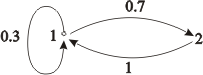
A diagram representing a two-state Markov process. The numbers are the probability of changing from one state to another state.

A Markov chain or Markov process is a stochastic model describing a sequence of possible events in which the probability of each event depends only on the state attained in the previous event.^[1]^[2]^[3] Informally, this may be thought of as, “What happens next depends only on the state of affairs now.” A countably infinite sequence, in which the chain moves state at discrete time steps, gives a discrete-time Markov chain (DTMC). A continuous-time process is called a continuous-time Markov chain (CTMC). It is named after the Russian mathematician Andrey Markov.

Markov chains have many applications as statistical models of real-world processes,^[1]^[4]^[5]^[6] such as studying cruise control systems in motor vehicles, queues or lines of customers arriving at an airport, currency exchange rates and animal population dynamics.^[7]

Markov processes are the basis for general stochastic simulation methods known as Markov chain Monte Carlo, which are used for simulating sampling from complex probability distributions, and have found application in Bayesian statistics, thermodynamics, statistical mechanics, physics, chemistry, economics, finance, signal processing, information theory and speech processing.^[7]^[8]^[9]

The adjectives Markovian and Markov are used to describe something that is related to a Markov process.^[1]^[10]^[11]

Principles[edit]

Definition[edit]

A Markov process is a stochastic process that satisfies the Markov property^[1] (sometimes characterized as “memorylessness”). In simpler terms, it is a process for which predictions can be made regarding future outcomes based solely on its present state and—most importantly—such predictions are just as good as the ones that could be made knowing the process’s full history.^[12] In other words, conditional on the present state of the system, its future and past states are independent.

A Markov chain is a type of Markov process that has either a discrete state space or a discrete index set (often representing time), but the precise definition of a Markov chain varies.^[13] For example, it is common to define a Markov chain as a Markov process in either discrete or continuous time with a countable state space (thus regardless of the nature of time),^[14]^[15]^[16]^[17] but it is also common to define a Markov chain as having discrete time in either countable or continuous state space (thus regardless of the state space).^[13]

Types of Markov chains[edit]

The system’s state space and time parameter index need to be specified. The following table gives an overview of the different instances of Markov processes for different levels of state space generality and for discrete time v. continuous time:

	Countable state space	Continuous or general state space
Discrete-time	(discrete-time) Markov chain on a countable or finite state space	Markov chain on a measurable state space (for example, Harris chain)
Continuous-time	Continuous-time Markov process or Markov jump process	Any continuous stochastic process with the Markov property (for example, the Wiener process)

Note that there is no definitive agreement in the literature on the use of some of the terms that signify special cases of Markov processes. Usually the term “Markov chain” is reserved for a process with a discrete set of times, that is, a discrete-time Markov chain (DTMC),^[1]^[18] but a few authors use the term “Markov process” to refer to a continuous-time Markov chain (CTMC) without explicit mention.^[19]^[20]^[21] In addition, there are other extensions of Markov processes that are referred to as such but do not necessarily fall within any of these four categories (see Markov model). Moreover, the time index need not necessarily be real-valued; like with the state space, there are conceivable processes that move through index sets with other mathematical constructs. Notice that the general state space continuous-time Markov chain is general to such a degree that it has no designated term.

While the time parameter is usually discrete, the state space of a Markov chain does not have any generally agreed-on restrictions: the term may refer to a process on an arbitrary state space.^[22] However, many applications of Markov chains employ finite or countably infinite state spaces, which have a more straightforward statistical analysis. Besides time-index and state-space parameters, there are many other variations, extensions and generalizations (see Variations). For simplicity, most of this article concentrates on the discrete-time, discrete state-space case, unless mentioned otherwise.

Transitions[edit]

The changes of state of the system are called transitions.^[1] The probabilities associated with various state changes are called transition probabilities. The process is characterized by a state space, a transition matrix describing the probabilities of particular transitions, and an initial state (or initial distribution) across the state space. By convention, we assume all possible states and transitions have been included in the definition of the process, so there is always a next state, and the process does not terminate.

A discrete-time random process involves a system which is in a certain state at each step, with the state changing randomly between steps.^[1] The steps are often thought of as moments in time, but they can equally well refer to physical distance or any other discrete measurement. Formally, the steps are the integers or natural numbers, and the random process is a mapping of these to states.^[23] The Markov property states that the conditional probability distribution for the system at the next step (and in fact at all future steps) depends only on the current state of the system, and not additionally on the state of the system at previous steps.

Since the system changes randomly, it is generally impossible to predict with certainty the state of a Markov chain at a given point in the future.^[23] However, the statistical properties of the system’s future can be predicted.^[23] In many applications, it is these statistical properties that are important.

History[edit]

Andrey Markov studied Markov processes in the early 20th century, publishing his first paper on the topic in 1906.^[24]^[25]^[26]^[27] Markov Processes in continuous time were discovered long before his work in the early 20th century^[1] in the form of the Poisson process.^[28]^[29]^[30] Markov was interested in studying an extension of independent random sequences, motivated by a disagreement with Pavel Nekrasov who claimed independence was necessary for the weak law of large numbers to hold.^[1]^[31] In his first paper on Markov chains, published in 1906, Markov showed that under certain conditions the average outcomes of the Markov chain would converge to a fixed vector of values, so proving a weak law of large numbers without the independence assumption,^[1]^[25]^[26]^[27] which had been commonly regarded as a requirement for such mathematical laws to hold.^[27] Markov later used Markov chains to study the distribution of vowels in Eugene Onegin, written by Alexander Pushkin, and proved a central limit theorem for such chains.^[1]^[25]

In 1912 Henri Poincaré studied Markov chains on finite groups with an aim to study card shuffling. Other early uses of Markov chains include a diffusion model, introduced by Paul and Tatyana Ehrenfest in 1907, and a branching process, introduced by Francis Galton and Henry William Watson in 1873, preceding the work of Markov.^[25]^[26] After the work of Galton and Watson, it was later revealed that their branching process had been independently discovered and studied around three decades earlier by Irénée-Jules Bienaymé.^[32] Starting in 1928, Maurice Fréchet became interested in Markov chains, eventually resulting in him publishing in 1938 a detailed study on Markov chains.^[25]^[33]

Andrey Kolmogorov developed in a 1931 paper a large part of the early theory of continuous-time Markov processes.^[34]^[35] Kolmogorov was partly inspired by Louis Bachelier’s 1900 work on fluctuations in the stock market as well as Norbert Wiener’s work on Einstein’s model of Brownian movement.^[34]^[36] He introduced and studied a particular set of Markov processes known as diffusion processes, where he derived a set of differential equations describing the processes.^[34]^[37] Independent of Kolmogorov’s work, Sydney Chapman derived in a 1928 paper an equation, now called the Chapman–Kolmogorov equation, in a less mathematically rigorous way than Kolmogorov, while studying Brownian movement.^[38] The differential equations are now called the Kolmogorov equations^[39] or the Kolmogorov–Chapman equations.^[40] Other mathematicians who contributed significantly to the foundations of Markov processes include William Feller, starting in 1930s, and then later Eugene Dynkin, starting in the 1950s.^[35]

Examples[edit]

Random walks based on integers and the gambler’s ruin problem are examples of Markov processes.^[41]^[42] Some variations of these processes were studied hundreds of years earlier in the context of independent variables.^[43]^[44]^[45] Two important examples of Markov processes are the Wiener process, also known as the Brownian motion process, and the Poisson process,^[28] which are considered the most important and central stochastic processes in the theory of stochastic processes.^[46]^[47]^[48] These two processes are Markov processes in continuous time, while random walks on the integers and the gambler’s ruin problem are examples of Markov processes in discrete time.^[41]^[42]
A famous Markov chain is the so-called “drunkard’s walk”, a random walk on the number line where, at each step, the position may change by +1 or −1 with equal probability. From any position there are two possible transitions, to the next or previous integer. The transition probabilities depend only on the current position, not on the manner in which the position was reached. For example, the transition probabilities from 5 to 4 and 5 to 6 are both 0.5, and all other transition probabilities from 5 are 0. These probabilities are independent of whether the system was previously in 4 or 6.
A series of independent states (for example, a series of coin flips) satisfies the formal definition of a Markov chain. However, the theory is usually applied only when the probability distribution of the next state depends on the current one.

A non-Markov example[edit]

Suppose that there is a coin purse containing five quarters (each worth 25¢), five dimes (each worth 10¢), and five nickels (each worth 5¢), and one by one, coins are randomly drawn from the purse and are set on a table. If $X_{n}$ represents the total value of the coins set on the table after n draws, with $X_{0}=0$ , then the sequence ${X_{n}:nin {mathbb {N}}}$ is not a Markov process.

To see why this is the case, suppose that in the first six draws, all five nickels and a quarter are drawn. Thus . If we know not just X_6 , but the earlier values as well, then we can determine which coins have been drawn, and we know that the next coin will not be a nickel; so we can determine that with probability 1. But if we do not know the earlier values, then based only on the value X_6 we might guess that we had drawn four dimes and two nickels, in which case it would certainly be possible to draw another nickel next. Thus, our guesses about X_7 are impacted by our knowledge of values prior to X_6 .

However, it is possible to model this scenario as a Markov process. Instead of defining $X_{n}$ to represent the total value of the coins on the table, we could define $X_{n}$ to represent the count of the various coin types on the table. For instance, ${displaystyle X_{6}=1,0,5}$ could be defined to represent the state where there is one quarter, zero dimes, and five nickels on the table after 6 one-by-one draws. This new model could be represented by possible states, where each state represents the number of coins of each type (from 0 to 5) that are on the table. (Not all of these states are reachable within 6 draws.) Suppose that the first draw results in state ${displaystyle X_{1}=0,1,0}$ . The probability of achieving $X_{2}$ now depends on $X_{1}$ ; for example, the state ${displaystyle X_{2}=1,0,1}$ is not possible. After the second draw, the third draw depends on which coins have so far been drawn, but no longer only on the coins that were drawn for the first state (since probabilistically important information has since been added to the scenario). In this way, the likelihood of the ${displaystyle X_{n}=i,j,k}$ state depends exclusively on the outcome of the ${displaystyle X_{n-1}=ell ,m,p}$ state.

Formal definition[edit]

Discrete-time Markov chain[edit]

A discrete-time Markov chain is a sequence of random variables X₁, X₂, X₃, … with the Markov property, namely that the probability of moving to the next state depends only on the present state and not on the previous states:

${displaystyle Pr(X_{n+1}=xmid X_{1}=x_{1},X_{2}=x_{2},ldots ,X_{n}=x_{n})=Pr(X_{n+1}=xmid X_{n}=x_{n}),}$

if both conditional probabilities are well defined, that is, if ${displaystyle Pr(X_{1}=x_{1},ldots ,X_{n}=x_{n})>0.}$

The possible values of X_i form a countable set S called the state space of the chain.

Variations[edit]

Continuous-time Markov chain[edit]

A continuous-time Markov chain (X_t)_t ≥ 0 is defined by a finite or countable state space S, a transition rate matrix Q with dimensions equal to that of the state space and initial probability distribution defined on the state space. For i ≠ j, the elements q_ij are non-negative and describe the rate of the process transitions from state i to state j. The elements q_ii are chosen such that each row of the transition rate matrix sums to zero, while the row-sums of a probability transition matrix in a (discrete) Markov chain are all equal to one.

There are three equivalent definitions of the process.^[49]

Infinitesimal definition[edit]

The continuous time Markov chain is characterized by the transition rates, the derivatives with respect to time of the transition probabilities between states i and j.

Let $X_{t}$ be the random variable describing the state of the process at time t, and assume the process is in a state i at time t.
Then, knowing ${displaystyle X_{t}=i}$ , ${displaystyle X_{t+h}=j}$ is independent of previous values ${displaystyle left(X_{s}:s<tright)}$ , and as h → 0 for all j and for all t,

${displaystyle Pr(X(t+h)=jmid X(t)=i)=delta _{ij}+q_{ij}h+o(h),}$

where $delta _{ij}$ is the Kronecker delta, using the little-o notation.
The $q_{ij}$ can be seen as measuring how quickly the transition from i to j happens.

Jump chain/holding time definition[edit]

Define a discrete-time Markov chain Y_n to describe the nth jump of the process and variables S₁, S₂, S₃, … to describe holding times in each of the states where S_i follows the exponential distribution with rate parameter −q_{Y_iY_i}.

Transition probability definition[edit]

For any value n = 0, 1, 2, 3, … and times indexed up to this value of n: t₀, t₁, t₂, … and all states recorded at these times i₀, i₁, i₂, i₃, … it holds that

${displaystyle Pr(X_{t_{n+1}}=i_{n+1}mid X_{t_{0}}=i_{0},X_{t_{1}}=i_{1},ldots ,X_{t_{n}}=i_{n})=p_{i_{n}i_{n+1}}(t_{n+1}-t_{n})}$

where p_ij is the solution of the forward equation (a first-order differential equation)

with initial condition P(0) is the identity matrix.

Finite state space[edit]

If the state space is finite, the transition probability distribution can be represented by a matrix, called the transition matrix, with the (i, j)th element of P equal to

${displaystyle p_{ij}=Pr(X_{n+1}=jmid X_{n}=i).}$

Since each row of P sums to one and all elements are non-negative, P is a right stochastic matrix.

Stationary distribution relation to eigenvectors and simplices[edit]

A stationary distribution π is a (row) vector, whose entries are non-negative and sum to 1, is unchanged by the operation of transition matrix P on it and so is defined by

By comparing this definition with that of an eigenvector we see that the two concepts are related and that

$pi ={frac {e}{sum _{i}{e_{i}}}}$

is a normalized ( ${textstyle sum _{i}pi _{i}=1}$ ) multiple of a left eigenvector e of the transition matrix P with an eigenvalue of 1. If there is more than one unit eigenvector then a weighted sum of the corresponding stationary states is also a stationary state. But for a Markov chain one is usually more interested in a stationary state that is the limit of the sequence of distributions for some initial distribution.

The values of a stationary distribution $textstyle pi _{i}$ are associated with the state space of P and its eigenvectors have their relative proportions preserved. Since the components of π are positive and the constraint that their sum is unity can be rewritten as ${textstyle sum _{i}1cdot pi _{i}=1}$ we see that the dot product of π with a vector whose components are all 1 is unity and that π lies on a simplex.

Time-homogeneous Markov chain with a finite state space[edit]

If the Markov chain is time-homogeneous, then the transition matrix P is the same after each step, so the k-step transition probability can be computed as the k-th power of the transition matrix, P^k.

If the Markov chain is irreducible and aperiodic, then there is a unique stationary distribution π.^[50] Additionally, in this case P^k converges to a rank-one matrix in which each row is the stationary distribution π:

${displaystyle lim _{kto infty }mathbf {P} ^{k}=mathbf {1} pi }$

where 1 is the column vector with all entries equal to 1. This is stated by the Perron–Frobenius theorem. If, by whatever means, ${textstyle lim _{kto infty }mathbf {P} ^{k}}$ is found, then the stationary distribution of the Markov chain in question can be easily determined for any starting distribution, as will be explained below.

For some stochastic matrices P, the limit ${textstyle lim _{kto infty }mathbf {P} ^{k}}$ does not exist while the stationary distribution does, as shown by this example:

${displaystyle mathbf {P} ={begin{pmatrix}0&1\1&0end{pmatrix}}qquad mathbf {P} ^{2k}=Iqquad mathbf {P} ^{2k+1}=mathbf {P} }$

${begin{pmatrix}{frac {1}{2}}&{frac {1}{2}}end{pmatrix}}{begin{pmatrix}0&1\1&0end{pmatrix}}={begin{pmatrix}{frac {1}{2}}&{frac {1}{2}}end{pmatrix}}$

(This example illustrates a periodic Markov chain.)

Because there are a number of different special cases to consider, the process of finding this limit if it exists can be a lengthy task. However, there are many techniques that can assist in finding this limit. Let P be an n×n matrix, and define ${textstyle mathbf {Q} =lim _{kto infty }mathbf {P} ^{k}.}$

It is always true that

Subtracting Q from both sides and factoring then yields

$mathbf {Q} (mathbf {P} -mathbf {I} _{n})=mathbf {0} _{n,n},$

where I_n is the identity matrix of size n, and 0_n,n is the zero matrix of size n×n. Multiplying together stochastic matrices always yields another stochastic matrix, so Q must be a stochastic matrix (see the definition above). It is sometimes sufficient to use the matrix equation above and the fact that Q is a stochastic matrix to solve for Q. Including the fact that the sum of each the rows in P is 1, there are n+1 equations for determining n unknowns, so it is computationally easier if on the one hand one selects one row in Q and substitutes each of its elements by one, and on the other one substitutes the corresponding element (the one in the same column) in the vector 0, and next left-multiplies this latter vector by the inverse of transformed former matrix to find Q.

Here is one method for doing so: first, define the function f(A) to return the matrix A with its right-most column replaced with all 1’s. If [f(P − I_n)]⁻¹ exists then^[51]^[50]

$mathbf {Q} =f(mathbf {0} _{n,n})[f(mathbf {P} -mathbf {I} _{n})]^{-1}.$

Explain: The original matrix equation is equivalent to a system of n×n linear equations in n×n variables. And there are n more linear equations from the fact that Q is a right stochastic matrix whose each row sums to 1. So it needs any n×n independent linear equations of the (n×n+n) equations to solve for the n×n variables. In this example, the n equations from “Q multiplied by the right-most column of (P-In)” have been replaced by the n stochastic ones.

One thing to notice is that if P has an element P_i,i on its main diagonal that is equal to 1 and the ith row or column is otherwise filled with 0’s, then that row or column will remain unchanged in all of the subsequent powers P^k. Hence, the ith row or column of Q will have the 1 and the 0’s in the same positions as in P.

Convergence speed to the stationary distribution[edit]

As stated earlier, from the equation (if exists) the stationary (or steady state) distribution π is a left eigenvector of row stochastic matrix P. Then assuming that P is diagonalizable or equivalently that P has n linearly independent eigenvectors, speed of convergence is elaborated as follows. (For non-diagonalizable, that is, defective matrices, one may start with the Jordan normal form of P and proceed with a bit more involved set of arguments in a similar way.^[52]

Let U be the matrix of eigenvectors (each normalized to having an L2 norm equal to 1) where each column is a left eigenvector of P and let Σ be the diagonal matrix of left eigenvalues of P, that is, Σ = diag(λ₁,λ₂,λ₃,…,λ_n). Then by eigendecomposition

$mathbf {P} =mathbf {USigma U} ^{-1}.$

Let the eigenvalues be enumerated such that:

${displaystyle 1=|lambda _{1}|>|lambda _{2}|geq |lambda _{3}|geq cdots geq |lambda _{n}|.}$

Since P is a row stochastic matrix, its largest left eigenvalue is 1. If there is a unique stationary distribution, then the largest eigenvalue and the corresponding eigenvector is unique too (because there is no other π which solves the stationary distribution equation above). Let u_i be the i-th column of U matrix, that is, u_i is the left eigenvector of P corresponding to λ_i. Also let x be a length n row vector that represents a valid probability distribution; since the eigenvectors u_i span ${displaystyle mathbb {R} ^{n},}$ we can write

${displaystyle mathbf {x} ^{mathsf {T}}=sum _{i=1}^{n}a_{i}mathbf {u} _{i},qquad a_{i}in mathbb {R} .}$

If we multiply x with P from right and continue this operation with the results, in the end we get the stationary distribution π. In other words, π = u_i ← xPP…P = xP^k as k → ∞. That means

${displaystyle {begin{aligned}{boldsymbol {pi }}^{(k)}&=mathbf {x} left(mathbf {USigma U} ^{-1}right)left(mathbf {USigma U} ^{-1}right)cdots left(mathbf {USigma U} ^{-1}right)\&=mathbf {xUSigma } ^{k}mathbf {U} ^{-1}\&=left(a_{1}mathbf {u} _{1}^{mathsf {T}}+a_{2}mathbf {u} _{2}^{mathsf {T}}+cdots +a_{n}mathbf {u} _{n}^{mathsf {T}}right)mathbf {USigma } ^{k}mathbf {U} ^{-1}\&=a_{1}lambda _{1}^{k}mathbf {u} _{1}^{mathsf {T}}+a_{2}lambda _{2}^{k}mathbf {u} _{2}^{mathsf {T}}+cdots +a_{n}lambda _{n}^{k}mathbf {u} _{n}^{mathsf {T}}&&u_{i}bot u_{j}{text{ for }}ineq j\&=lambda _{1}^{k}left{a_{1}mathbf {u} _{1}^{mathsf {T}}+a_{2}left({frac {lambda _{2}}{lambda _{1}}}right)^{k}mathbf {u} _{2}^{mathsf {T}}+a_{3}left({frac {lambda _{3}}{lambda _{1}}}right)^{k}mathbf {u} _{3}^{mathsf {T}}+cdots +a_{n}left({frac {lambda _{n}}{lambda _{1}}}right)^{k}mathbf {u} _{n}^{mathsf {T}}right}end{aligned}}}$

Since π = u₁, π^(k) approaches to π as k → ∞ with a speed in the order of λ₂/λ₁ exponentially. This follows because ${displaystyle |lambda _{2}|geq cdots geq |lambda _{n}|,}$ hence λ₂/λ₁ is the dominant term. The smaller the ratio is, the faster the convergence is.^[53] Random noise in the state distribution π can also speed up this convergence to the stationary distribution.^[54]

General state space[edit]

Harris chains[edit]

Many results for Markov chains with finite state space can be generalized to chains with uncountable state space through Harris chains.

The use of Markov chains in Markov chain Monte Carlo methods covers cases where the process follows a continuous state space.

Locally interacting Markov chains[edit]

Considering a collection of Markov chains whose evolution takes in account the state of other Markov chains, is related to the notion of locally interacting Markov chains. This corresponds to the situation when the state space has a (Cartesian-) product form.
See interacting particle system and stochastic cellular automata (probabilistic cellular automata).
See for instance Interaction of Markov Processes^[55]
or.^[56]

Properties[edit]

Two states are said to communicate with each other if both are reachable from one another by a sequence of transitions that have positive probability. This is an equivalence relation which yields a set of communicating classes. A class is closed if the probability of leaving the class is zero. A Markov chain is irreducible if there is one communicating class, the state space.

A state i has period k if k is the greatest common divisor of the number of transitions by which i can be reached, starting from i. That is:

$k=gcd{n>0:Pr(X_{n}=imid X_{0}=i)>0}$

A state i is said to be transient if, starting from i, there is a non-zero probability that the chain will never return to i. It is called recurrent (or persistent) otherwise.^[57] For a recurrent state i, the mean hitting time is defined as:

${displaystyle M_{i}=E[T_{i}]=sum _{n=1}^{infty }ncdot f_{ii}^{(n)}.}$

State i is positive recurrent if $M_{i}$ is finite and null recurrent otherwise. Periodicity, transience, recurrence and positive and null recurrence are class properties — that is, if one state has the property then all states in its communicating class have the property.

A state i is called absorbing if there are no outgoing transitions from the state.

Ergodicity[edit]

A state i is said to be ergodic if it is aperiodic and positive recurrent. In other words, a state i is ergodic if it is recurrent, has a period of 1, and has finite mean recurrence time. If all states in an irreducible Markov chain are ergodic, then the chain is said to be ergodic. Some authors call any irreducible, positive recurrent Markov chains ergodic, even periodic ones.^[58]

It can be shown that a finite state irreducible Markov chain is ergodic if it has an aperiodic state. More generally, a Markov chain is ergodic if there is a number N such that any state can be reached from any other state in any number of steps less or equal to a number N. In case of a fully connected transition matrix, where all transitions have a non-zero probability, this condition is fulfilled with N = 1.

A Markov chain with more than one state and just one out-going transition per state is either not irreducible or not aperiodic, hence cannot be ergodic.

Markovian representations[edit]

In some cases, apparently non-Markovian processes may still have Markovian representations, constructed by expanding the concept of the “current” and “future” states. For example, let X be a non-Markovian process. Then define a process Y, such that each state of Y represents a time-interval of states of X. Mathematically, this takes the form:

Y(t) = big{ X(s): s in [a(t), b(t)] , big}.

If Y has the Markov property, then it is a Markovian representation of X.

An example of a non-Markovian process with a Markovian representation is an autoregressive time series of order greater than one.^[59]

Hitting times[edit]

The hitting time is the time, starting in a given set of states until the chain arrives in a given state or set of states. The distribution of such a time period has a phase type distribution. The simplest such distribution is that of a single exponentially distributed transition.

Expected hitting times[edit]

For a subset of states A ⊆ S, the vector k^A of hitting times (where element ${displaystyle k_{i}^{A}}$ represents the expected value, starting in state i that the chain enters one of the states in the set A) is the minimal non-negative solution to^[60]

${displaystyle begin{align} k_i^A = 0 & text{ for } i in A\ -sum_{j in S} q_{ij} k_j^A = 1&text{ for } i notin A. end{align}}$

Time reversal[edit]

For a CTMC X_t, the time-reversed process is defined to be ${displaystyle {hat {X}}_{t}=X_{T-t}}$ . By Kelly’s lemma this process has the same stationary distribution as the forward process.

A chain is said to be reversible if the reversed process is the same as the forward process. Kolmogorov’s criterion states that the necessary and sufficient condition for a process to be reversible is that the product of transition rates around a closed loop must be the same in both directions.

Embedded Markov chain[edit]

One method of finding the stationary probability distribution, π, of an ergodic continuous-time Markov chain, Q, is by first finding its embedded Markov chain (EMC). Strictly speaking, the EMC is a regular discrete-time Markov chain, sometimes referred to as a jump process. Each element of the one-step transition probability matrix of the EMC, S, is denoted by s_ij, and represents the conditional probability of transitioning from state i into state j. These conditional probabilities may be found by

${displaystyle s_{ij} = begin{cases} frac{q_{ij}}{sum_{k neq i} q_{ik}} & text{if } i neq j \ 0 & text{otherwise}. end{cases} }$

From this, S may be written as

${displaystyle S = I - left( operatorname{diag}(Q) right)^{-1} Q}$

where I is the identity matrix and diag(Q) is the diagonal matrix formed by selecting the main diagonal from the matrix Q and setting all other elements to zero.

To find the stationary probability distribution vector, we must next find varphi such that

with varphi being a row vector, such that all elements in varphi are greater than 0 and ${displaystyle |varphi |_{1}}$ = 1. From this, π may be found as

${displaystyle pi ={-varphi (operatorname {diag} (Q))^{-1} over left|varphi (operatorname {diag} (Q))^{-1}right|_{1}}.}$

(S may be periodic, even if Q is not. Once π is found, it must be normalized to a unit vector.)

Another discrete-time process that may be derived from a continuous-time Markov chain is a δ-skeleton—the (discrete-time) Markov chain formed by observing X(t) at intervals of δ units of time. The random variables X(0), X(δ), X(2δ), … give the sequence of states visited by the δ-skeleton.

Special types of Markov chains[edit]

Markov model[edit]

Markov models are used to model changing systems. There are 4 main types of models, that generalize Markov chains depending on whether every sequential state is observable or not, and whether the system is to be adjusted on the basis of observations made:

	System state is fully observable	System state is partially observable
System is autonomous	Markov chain	Hidden Markov model
System is controlled	Markov decision process	Partially observable Markov decision process

Bernoulli scheme[edit]

A Bernoulli scheme is a special case of a Markov chain where the transition probability matrix has identical rows, which means that the next state is independent of even the current state (in addition to being independent of the past states). A Bernoulli scheme with only two possible states is known as a Bernoulli process.

Note, however, by the Ornstein isomorphism theorem, that every aperiodic and irreducible Markov chain is isomorphic to a Bernoulli scheme;^[61] thus, one might equally claim that Markov chains are a “special case” of Bernoulli schemes. The isomorphism generally requires a complicated recoding. The isomorphism theorem is even a bit stronger: it states that any stationary stochastic process is isomorphic to a Bernoulli scheme; the Markov chain is just one such example.

Subshift of finite type[edit]

When the Markov matrix is replaced by the adjacency matrix of a finite graph, the resulting shift is termed a topological Markov chain or a subshift of finite type.^[61] A Markov matrix that is compatible with the adjacency matrix can then provide a measure on the subshift. Many chaotic dynamical systems are isomorphic to topological Markov chains; examples include diffeomorphisms of closed manifolds, the Prouhet–Thue–Morse system, the Chacon system, sofic systems, context-free systems and block-coding systems.^[61]

Applications[edit]

Research has reported the application and usefulness of Markov chains in a wide range of topics such as physics, chemistry, biology, medicine, music, game theory and sports.

Physics[edit]

Markovian systems appear extensively in thermodynamics and statistical mechanics, whenever probabilities are used to represent unknown or unmodelled details of the system, if it can be assumed that the dynamics are time-invariant, and that no relevant history need be considered which is not already included in the state description.^[62]^[63] For example, a thermodynamic state operates under a probability distribution that is difficult or expensive to acquire. Therefore, Markov Chain Monte Carlo method can be used to draw samples randomly from a black-box to approximate the probability distribution of attributes over a range of objects.^[63]

The paths, in the path integral formulation of quantum mechanics, are Markov chains.^[64]

Markov chains are used in lattice QCD simulations.^[65]

Chemistry[edit]

Michaelis-Menten kinetics. The enzyme (E) binds a substrate (S) and produces a product (P). Each reaction is a state transition in a Markov chain.

A reaction network is a chemical system involving multiple reactions and chemical species. The simplest stochastic models of such networks treat the system as a continuous time Markov chain with the state being the number of molecules of each species and with reactions modeled as possible transitions of the chain.^[66] Markov chains and continuous-time Markov processes are useful in chemistry when physical systems closely approximate the Markov property. For example, imagine a large number n of molecules in solution in state A, each of which can undergo a chemical reaction to state B with a certain average rate. Perhaps the molecule is an enzyme, and the states refer to how it is folded. The state of any single enzyme follows a Markov chain, and since the molecules are essentially independent of each other, the number of molecules in state A or B at a time is n times the probability a given molecule is in that state.

The classical model of enzyme activity, Michaelis–Menten kinetics, can be viewed as a Markov chain, where at each time step the reaction proceeds in some direction. While Michaelis-Menten is fairly straightforward, far more complicated reaction networks can also be modeled with Markov chains.^[67]

An algorithm based on a Markov chain was also used to focus the fragment-based growth of chemicals in silico towards a desired class of compounds such as drugs or natural products.^[68] As a molecule is grown, a fragment is selected from the nascent molecule as the “current” state. It is not aware of its past (that is, it is not aware of what is already bonded to it). It then transitions to the next state when a fragment is attached to it. The transition probabilities are trained on databases of authentic classes of compounds.^[69]

Also, the growth (and composition) of copolymers may be modeled using Markov chains. Based on the reactivity ratios of the monomers that make up the growing polymer chain, the chain’s composition may be calculated (for example, whether monomers tend to add in alternating fashion or in long runs of the same monomer). Due to steric effects, second-order Markov effects may also play a role in the growth of some polymer chains.

Similarly, it has been suggested that the crystallization and growth of some epitaxial superlattice oxide materials can be accurately described by Markov chains.^[70]

Biology[edit]

Markov chains are used in various areas of biology. Notable examples include:

Phylogenetics and bioinformatics, where most models of DNA evolution use continuous-time Markov chains to describe the nucleotide present at a given site in the genome.
Population dynamics, where Markov chains are in particular a central tool in the theoretical study of matrix population models.
Neurobiology, where Markov chains have been used, e.g., to simulate the mammalian neocortex.^[71]
Systems biology, for instance with the modeling of viral infection of single cells.^[72]
Compartmental models for disease outbreak and epidemic modeling.

Testing[edit]

Several theorists have proposed the idea of the Markov chain statistical test (MCST), a method of conjoining Markov chains to form a “Markov blanket”, arranging these chains in several recursive layers (“wafering”) and producing more efficient test sets—samples—as a replacement for exhaustive testing. MCSTs also have uses in temporal state-based networks; Chilukuri et al.’s paper entitled “Temporal Uncertainty Reasoning Networks for Evidence Fusion with Applications to Object Detection and Tracking” (ScienceDirect) gives a background and case study for applying MCSTs to a wider range of applications.

Solar irradiance variability[edit]

Solar irradiance variability assessments are useful for solar power applications. Solar irradiance variability at any location over time is mainly a consequence of the deterministic variability of the sun’s path across the sky dome and the variability in cloudiness. The variability of accessible solar irradiance on Earth’s surface has been modeled using Markov chains,^[73]^[74]^[75]^[76] also including modeling the two states of clear and cloudiness as a two-state Markov chain.^[77]^[78]

Speech recognition[edit]

Hidden Markov models are the basis for most modern automatic speech recognition systems.

Information theory[edit]

Markov chains are used throughout information processing. Claude Shannon’s famous 1948 paper A Mathematical Theory of Communication, which in a single step created the field of information theory, opens by introducing the concept of entropy through Markov modeling of the English language. Such idealized models can capture many of the statistical regularities of systems. Even without describing the full structure of the system perfectly, such signal models can make possible very effective data compression through entropy encoding techniques such as arithmetic coding. They also allow effective state estimation and pattern recognition. Markov chains also play an important role in reinforcement learning.

Markov chains are also the basis for hidden Markov models, which are an important tool in such diverse fields as telephone networks (which use the Viterbi algorithm for error correction), speech recognition and bioinformatics (such as in rearrangements detection^[79]).

The LZMA lossless data compression algorithm combines Markov chains with Lempel-Ziv compression to achieve very high compression ratios.

Queueing theory[edit]

Markov chains are the basis for the analytical treatment of queues (queueing theory). Agner Krarup Erlang initiated the subject in 1917.^[80] This makes them critical for optimizing the performance of telecommunications networks, where messages must often compete for limited resources (such as bandwidth).^[81]

Numerous queueing models use continuous-time Markov chains. For example, an M/M/1 queue is a CTMC on the non-negative integers where upward transitions from i to i + 1 occur at rate λ according to a Poisson process and describe job arrivals, while transitions from i to i – 1 (for i > 1) occur at rate μ (job service times are exponentially distributed) and describe completed services (departures) from the queue.

Internet applications[edit]

A state diagram that represents the PageRank algorithm with a transitional probability of M, or ${frac {alpha }{k_{i}}}+{frac {1-alpha }{N}}$ .

The PageRank of a webpage as used by Google is defined by a Markov chain.^[82]^[83]^[84] It is the probability to be at page in the stationary distribution on the following Markov chain on all (known) webpages. If is the number of known webpages, and a page has $k_{i}$ links to it then it has transition probability ${frac {alpha }{k_{i}}}+{frac {1-alpha }{N}}$ for all pages that are linked to and ${frac {1-alpha }{N}}$ for all pages that are not linked to. The parameter alpha is taken to be about 0.15.

Markov models have also been used to analyze web navigation behavior of users. A user’s web link transition on a particular website can be modeled using first- or second-order Markov models and can be used to make predictions regarding future navigation and to personalize the web page for an individual user.

Statistics[edit]

Markov chain methods have also become very important for generating sequences of random numbers to accurately reflect very complicated desired probability distributions, via a process called Markov chain Monte Carlo (MCMC). In recent years this has revolutionized the practicability of Bayesian inference methods, allowing a wide range of posterior distributions to be simulated and their parameters found numerically.

Economics and finance[edit]

Markov chains are used in finance and economics to model a variety of different phenomena, including the distribution of income, the size distribution of firms, asset prices and market crashes. D. G. Champernowne built a Markov chain model of the distribution of income in 1953.^[86] Herbert A. Simon and co-author Charles Bonini used a Markov chain model to derive a stationary Yule distribution of firm sizes.^[87] Louis Bachelier was the first to observe that stock prices followed a random walk.^[88] The random walk was later seen as evidence in favor of the efficient-market hypothesis and random walk models were popular in the literature of the 1960s.^[89] Regime-switching models of business cycles were popularized by James D. Hamilton (1989), who used a Markov chain to model switches between periods of high and low GDP growth (or, alternatively, economic expansions and recessions).^[90] A more recent example is the Markov switching multifractal model of Laurent E. Calvet and Adlai J. Fisher, which builds upon the convenience of earlier regime-switching models.^[91]^[92] It uses an arbitrarily large Markov chain to drive the level of volatility of asset returns.

Dynamic macroeconomics makes heavy use of Markov chains. An example is using Markov chains to exogenously model prices of equity (stock) in a general equilibrium setting.^[93]

Credit rating agencies produce annual tables of the transition probabilities for bonds of different credit ratings.^[94]

[edit]

Markov chains are generally used in describing path-dependent arguments, where current structural configurations condition future outcomes. An example is the reformulation of the idea, originally due to Karl Marx’s Das Kapital, tying economic development to the rise of capitalism. In current research, it is common to use a Markov chain to model how once a country reaches a specific level of economic development, the configuration of structural factors, such as size of the middle class, the ratio of urban to rural residence, the rate of political mobilization, etc., will generate a higher probability of transitioning from authoritarian to democratic regime.^[95]

Games[edit]

Markov chains can be used to model many games of chance.^[1] The children’s games Snakes and Ladders and “Hi Ho! Cherry-O”, for example, are represented exactly by Markov chains. At each turn, the player starts in a given state (on a given square) and from there has fixed odds of moving to certain other states (squares).

Music[edit]

Markov chains are employed in algorithmic music composition, particularly in software such as Csound, Max, and SuperCollider. In a first-order chain, the states of the system become note or pitch values, and a probability vector for each note is constructed, completing a transition probability matrix (see below). An algorithm is constructed to produce output note values based on the transition matrix weightings, which could be MIDI note values, frequency (Hz), or any other desirable metric.^[96]

1st-order matrix

Note	A	C♯	E♭
A	0.1	0.6	0.3
C♯	0.25	0.05	0.7
E♭	0.7	0.3	0

2nd-order matrix

Notes	A	D	G
AA	0.18	0.6	0.22
AD	0.5	0.5	0
AG	0.15	0.75	0.1
DD	0	0	1
DA	0.25	0	0.75
DG	0.9	0.1	0
GG	0.4	0.4	0.2
GA	0.5	0.25	0.25
GD	1	0	0

A second-order Markov chain can be introduced by considering the current state and also the previous state, as indicated in the second table. Higher, nth-order chains tend to “group” particular notes together, while ‘breaking off’ into other patterns and sequences occasionally. These higher-order chains tend to generate results with a sense of phrasal structure, rather than the ‘aimless wandering’ produced by a first-order system.^[97]

Markov chains can be used structurally, as in Xenakis’s Analogique A and B.^[98] Markov chains are also used in systems which use a Markov model to react interactively to music input.^[99]

Usually musical systems need to enforce specific control constraints on the finite-length sequences they generate, but control constraints are not compatible with Markov models, since they induce long-range dependencies that violate the Markov hypothesis of limited memory. In order to overcome this limitation, a new approach has been proposed.^[100]

Baseball[edit]

Markov chain models have been used in advanced baseball analysis since 1960, although their use is still rare. Each half-inning of a baseball game fits the Markov chain state when the number of runners and outs are considered. During any at-bat, there are 24 possible combinations of number of outs and position of the runners. Mark Pankin shows that Markov chain models can be used to evaluate runs created for both individual players as well as a team.^[101]
He also discusses various kinds of strategies and play conditions: how Markov chain models have been used to analyze statistics for game situations such as bunting and base stealing and differences when playing on grass vs. AstroTurf.^[102]

Markov text generators[edit]

Markov processes can also be used to generate superficially real-looking text given a sample document. Markov processes are used in a variety of recreational “parody generator” software (see dissociated press, Jeff Harrison,^[103] Mark V. Shaney,^[104]^[105] and Academias Neutronium). Several open-source text generation libraries using Markov chains exist, including The RiTa Toolkit.

Probabilistic forecasting[edit]

Markov chains have been used for forecasting in several areas: for example, price trends,^[106] wind power,^[107] and solar irradiance.^[108] The Markov chain forecasting models utilize a variety of settings, from discretizing the time series,^[107] to hidden Markov models combined with wavelets,^[106] and the Markov chain mixture distribution model (MCM).^[108]

Notes[edit]

^ ^a ^b ^c ^d ^e ^f ^g ^h ⁱ ^j ^k ^l Gagniuc, Paul A. (2017). Markov Chains: From Theory to Implementation and Experimentation. USA, NJ: John Wiley & Sons. pp. 1–235. ISBN 978-1-119-38755-8.
^ “Markov chain | Definition of Markov chain in US English by Oxford Dictionaries”. Oxford Dictionaries. Archived from the original on December 15, 2017. Retrieved 2017-12-14.
^ Definition at Brilliant.org “Brilliant Math and Science Wiki”. Retrieved on 12 May 2019
^ Samuel Karlin; Howard E. Taylor (2 December 2012). A First Course in Stochastic Processes. Academic Press. p. 47. ISBN 978-0-08-057041-9. Archived from the original on 23 March 2017.
^ Bruce Hajek (12 March 2015). Random Processes for Engineers. Google Books. Cambridge University Press. ISBN 978-1-316-24124-0. Archived from the original on 23 March 2017.
^ G. Latouche; V. Ramaswami (1 January 1999). Introduction to Matrix Analytic Methods in Stochastic Modeling. SIAM. pp. 4–. ISBN 978-0-89871-425-8. Archived from the original on 23 March 2017.
^ ^a ^b Sean Meyn; Richard L. Tweedie (2 April 2009). Markov Chains and Stochastic Stability. Cambridge University Press. p. 3. ISBN 978-0-521-73182-9. Archived from the original on 23 March 2017.
^ Reuven Y. Rubinstein; Dirk P. Kroese (20 September 2011). Simulation and the Monte Carlo Method. John Wiley & Sons. p. 225. ISBN 978-1-118-21052-9. Archived from the original on 23 March 2017.
^ Dani Gamerman; Hedibert F. Lopes (10 May 2006). Markov Chain Monte Carlo: Stochastic Simulation for Bayesian Inference, Second Edition. CRC Press. ISBN 978-1-58488-587-0. Archived from the original on 23 March 2017.
^ “Markovian”. Oxford English Dictionary (Online ed.). Oxford University Press. (Subscription or participating institution membership required.)
^ Model-Based Signal Processing. John Wiley & Sons. 27 October 2005. ISBN 9780471732662.
^ Øksendal, B. K. (Bernt Karsten) (2003). Stochastic differential equations : an introduction with applications (6th ed.). Berlin: Springer. ISBN 3540047581. OCLC 52203046.
^ ^a ^b Søren Asmussen (15 May 2003). Applied Probability and Queues. Springer Science & Business Media. p. 7. ISBN 978-0-387-00211-8. Archived from the original on 23 March 2017.
^ Emanuel Parzen (17 June 2015). Stochastic Processes. Courier Dover Publications. p. 188. ISBN 978-0-486-79688-8. Archived from the original on 20 November 2017.
^ Samuel Karlin; Howard E. Taylor (2 December 2012). A First Course in Stochastic Processes. Academic Press. pp. 29 and 30. ISBN 978-0-08-057041-9. Archived from the original on 23 March 2017.
^ John Lamperti (1977). Stochastic processes: a survey of the mathematical theory. Springer-Verlag. pp. 106–121. ISBN 978-3-540-90275-1. Archived from the original on 2017-03-23.
^ Sheldon M. Ross (1996). Stochastic processes. Wiley. pp. 174 and 231. ISBN 978-0-471-12062-9. Archived from the original on 2017-03-23.
^ Everitt, B.S. (2002) The Cambridge Dictionary of Statistics. CUP. ISBN 0-521-81099-X
^ Parzen, E. (1962) Stochastic Processes, Holden-Day. ISBN 0-8162-6664-6 (Table 6.1)
^ Dodge, Y. (2003) The Oxford Dictionary of Statistical Terms, OUP. ISBN 0-19-920613-9 (entry for “Markov chain”)
^ Dodge, Y. The Oxford Dictionary of Statistical Terms, OUP. ISBN 0-19-920613-9
^ Meyn, S. Sean P., and Richard L. Tweedie. (2009) Markov chains and stochastic stability. Cambridge University Press. (Preface, p. iii)
^ ^a ^b ^c Gagniuc, Paul A. (2017). Markov Chains: From Theory to Implementation and Experimentation. USA, NJ: John Wiley & Sons. pp. 159–163. ISBN 978-1-119-38755-8.
^ Gagniuc, Paul A. (2017). Markov Chains: From Theory to Implementation and Experimentation. USA, NJ: John Wiley & Sons. pp. 2–8. ISBN 978-1-119-38755-8.
^ ^a ^b ^c ^d ^e Charles Miller Grinstead; James Laurie Snell (1997). Introduction to Probability. American Mathematical Soc. pp. 464–466. ISBN 978-0-8218-0749-1.
^ ^a ^b ^c Pierre Bremaud (9 March 2013). Markov Chains: Gibbs Fields, Monte Carlo Simulation, and Queues. Springer Science & Business Media. p. ix. ISBN 978-1-4757-3124-8. Archived from the original on 23 March 2017.
^ ^a ^b ^c Hayes, Brian (2013). “First links in the Markov chain”. American Scientist. 101 (2): 92–96. doi:10.1511/2013.101.92.
^ ^a ^b Sheldon M. Ross (1996). Stochastic processes. Wiley. pp. 235 and 358. ISBN 978-0-471-12062-9. Archived from the original on 2017-03-23.
^ Jarrow, Robert; Protter, Philip (2004). “A short history of stochastic integration and mathematical finance: The early years, 1880–1970”. A Festschrift for Herman Rubin. Institute of Mathematical Statistics Lecture Notes – Monograph Series. pp. 75–91. CiteSeerX 10.1.1.114.632. doi:10.1214/lnms/1196285381. ISBN 978-0-940600-61-4. ISSN 0749-2170.
^ Guttorp, Peter; Thorarinsdottir, Thordis L. (2012). “What Happened to Discrete Chaos, the Quenouille Process, and the Sharp Markov Property? Some History of Stochastic Point Processes”. International Statistical Review. 80 (2): 253–268. doi:10.1111/j.1751-5823.2012.00181.x. ISSN 0306-7734. S2CID 80836.
^ Seneta, E. (1996). “Markov and the Birth of Chain Dependence Theory”. International Statistical Review / Revue Internationale de Statistique. 64 (3): 255–257. doi:10.2307/1403785. ISSN 0306-7734. JSTOR 1403785.
^ Seneta, E. (1998). “I.J. Bienaymé [1796–1878]: Criticality, Inequality, and Internationalization”. International Statistical Review / Revue Internationale de Statistique. 66 (3): 291–292. doi:10.2307/1403518. ISSN 0306-7734. JSTOR 1403518.
^ Bru B, Hertz S (2001). “Maurice Fréchet”. In Heyde CC, Seneta E, Crépel P, Fienberg SE, Gani J (eds.). Statisticians of the Centuries. New York, NY: Springer. pp. 331–334. doi:10.1007/978-1-4613-0179-0_71. ISBN 978-0-387-95283-3.
^ ^a ^b ^c Kendall, D. G.; Batchelor, G. K.; Bingham, N. H.; Hayman, W. K.; Hyland, J. M. E.; Lorentz, G. G.; Moffatt, H. K.; Parry, W.; Razborov, A. A.; Robinson, C. A.; Whittle, P. (1990). “Andrei Nikolaevich Kolmogorov (1903–1987)”. Bulletin of the London Mathematical Society. 22 (1): 33. doi:10.1112/blms/22.1.31. ISSN 0024-6093.
^ ^a ^b Cramér, Harald (1976). “Half a Century with Probability Theory: Some Personal Recollections”. The Annals of Probability. 4 (4): 509–546. doi:10.1214/aop/1176996025. ISSN 0091-1798.
^ Marc Barbut; Bernard Locker; Laurent Mazliak (23 August 2016). Paul Lévy and Maurice Fréchet: 50 Years of Correspondence in 107 Letters. Springer London. p. 5. ISBN 978-1-4471-7262-8. Archived from the original on 23 March 2017.
^ Valeriy Skorokhod (5 December 2005). Basic Principles and Applications of Probability Theory. Springer Science & Business Media. p. 146. ISBN 978-3-540-26312-8. Archived from the original on 23 March 2017.
^ Bernstein, Jeremy (2005). “Bachelier”. American Journal of Physics. 73 (5): 395–398. Bibcode:2005AmJPh..73..395B. doi:10.1119/1.1848117. ISSN 0002-9505.
^ William J. Anderson (6 December 2012). Continuous-Time Markov Chains: An Applications-Oriented Approach. Springer Science & Business Media. p. vii. ISBN 978-1-4612-3038-0. Archived from the original on 23 March 2017.
^ Kendall, D. G.; Batchelor, G. K.; Bingham, N. H.; Hayman, W. K.; Hyland, J. M. E.; Lorentz, G. G.; Moffatt, H. K.; Parry, W.; Razborov, A. A.; Robinson, C. A.; Whittle, P. (1990). “Andrei Nikolaevich Kolmogorov (1903–1987)”. Bulletin of the London Mathematical Society. 22 (1): 57. doi:10.1112/blms/22.1.31. ISSN 0024-6093.
^ ^a ^b Ionut Florescu (7 November 2014). Probability and Stochastic Processes. John Wiley & Sons. pp. 373 and 374. ISBN 978-1-118-59320-2. Archived from the original on 23 March 2017.
^ ^a ^b Samuel Karlin; Howard E. Taylor (2 December 2012). A First Course in Stochastic Processes. Academic Press. p. 49. ISBN 978-0-08-057041-9. Archived from the original on 23 March 2017.
^ Gagniuc, Paul A. (2017). Markov Chains: From Theory to Implementation and Experimentation. USA, NJ: John Wiley & Sons. pp. 1–2. ISBN 978-1-119-38755-8.
^ Weiss, George H. (2006). “Random Walks”. Encyclopedia of Statistical Sciences. p. 1. doi:10.1002/0471667196.ess2180.pub2. ISBN 978-0471667193.
^ Michael F. Shlesinger (1985). The Wonderful world of stochastics: a tribute to Elliott W. Montroll. North-Holland. pp. 8–10. ISBN 978-0-444-86937-1. Archived from the original on 2017-03-23.
^ Emanuel Parzen (17 June 2015). Stochastic Processes. Courier Dover Publications. p. 7 and 8. ISBN 978-0-486-79688-8. Archived from the original on 20 November 2017.
^ Joseph L. Doob (1990). Stochastipoic processes. Wiley. p. 46 and 47. Archived from the original on 2017-11-20.
^ Donald L. Snyder; Michael I. Miller (6 December 2012). Random Point Processes in Time and Space. Springer Science & Business Media. p. 32. ISBN 978-1-4612-3166-0. Archived from the original on 20 November 2017.
^ Norris, J. R. (1997). “Continuous-time Markov chains I”. Markov Chains. pp. 60–107. doi:10.1017/CBO9780511810633.004. ISBN 9780511810633.
^ ^a ^b Serfozo, Richard (2009). “Basics of Applied Stochastic Processes”. Probability and Its Applications. doi:10.1007/978-3-540-89332-5. ISBN 978-3-540-89331-8. ISSN 1431-7028.
^ “Chapter 11 “Markov Chains”” (PDF). Archived (PDF) from the original on 2017-02-15. Retrieved 2017-06-02.
^ Schmitt, Florian; Rothlauf, Franz (2001). “On the Importance of the Second Largest Eigenvalue on the Convergence Rate of Genetic Algorithms”. Proceedings of the 14th Symposium on Reliable Distributed Systems. CiteSeerX 10.1.1.28.6191.
^ Rosenthal, Jeffrey S. (1995). “Convergence Rates for Markov Chains”. SIAM Review. 37 (3): 387–405. doi:10.1137/1037083. ISSN 0036-1445. JSTOR 2132659. Retrieved 2021-05-31.
^ Franzke, Brandon; Kosko, Bart (1 October 2011). “Noise can speed convergence in Markov chains”. Physical Review E. 84 (4): 041112. Bibcode:2011PhRvE..84d1112F. doi:10.1103/PhysRevE.84.041112. PMID 22181092.
^ Spitzer, Frank (1970). “Interaction of Markov Processes”. Advances in Mathematics. 5 (2): 246–290. doi:10.1016/0001-8708(70)90034-4.
^ Dobrushin, R. L.; Kryukov, V. I.; Toom, A. L. (1978). Stochastic Cellular Systems: Ergodicity, Memory, Morphogenesis. ISBN 9780719022067. Archived from the original on 2017-02-05. Retrieved 2016-03-04.
^ Heyman, Daniel P.; Sobel, Mathew J. (1982). Stochastic Models in Operations Research, Volume 1. New York: McGraw-Hill. p. 230. ISBN 0-07-028631-0.
^ Parzen, Emanuel (1962). Stochastic Processes. San Francisco: Holden-Day. p. 145. ISBN 0-8162-6664-6.
^ Doblinger, G. (September 1998). “Smoothing of noisy AR signals using an adaptive Kalman filter” (PDF). 9th European Signal Processing Conference (EUSIPCO 1998): 781–784.
^ Norris, J. R. (1997). “Continuous-time Markov chains II”. Markov Chains. pp. 108–127. doi:10.1017/CBO9780511810633.005. ISBN 9780511810633.
^ ^a ^b ^c
Matthew Nicol and Karl Petersen, (2009) “Ergodic Theory: Basic Examples and Constructions”,
Encyclopedia of Complexity and Systems Science, Springer https://doi.org/10.1007/978-0-387-30440-3_177
^ Fitzpatrick, Richard. “Thermodynamics and Statistical Mechanics” (PDF). Archived (PDF) from the original on 2016-11-30. Retrieved 2017-06-02.
^ ^a ^b van Ravenzwaaij, Don; Cassey, Pete; Brown, Scott D. (2016-03-11). “A simple introduction to Markov Chain Monte–Carlo sampling”. Psychonomic Bulletin & Review. 25 (1): 143–154. doi:10.3758/s13423-016-1015-8. ISSN 1069-9384. PMC 5862921. PMID 26968853.
^ Ryder, Lewis H. (1985). Quantum field theory. Cambridge [Cambridgeshire]: Cambridge University Press. pp. 160. ISBN 978-0521338592. OCLC 10533049.
^ Gattringer, Christof; Lang, Christian B (2010). Quantum Chromodynamics on the Lattice. Lecture Notes in Physics. Vol. 788. Springer-Verlag Berlin Heidelberg. doi:10.1007/978-3-642-01850-3. ISBN 978-3-642-01849-7. Archived from the original on 2017-08-01.
^ Anderson, David F.; Kurtz, Thomas G. (2011), “Continuous Time Markov Chain Models for Chemical Reaction Networks”, Design and Analysis of Biomolecular Circuits, Springer New York, pp. 3–42, doi:10.1007/978-1-4419-6766-4_1, ISBN 9781441967657
^ Du, Chao; Kou, S. C. (September 2012). “Correlation analysis of enzymatic reaction of a single protein molecule”. The Annals of Applied Statistics. 6 (3): 950–976. arXiv:1209.6210. Bibcode:2012arXiv1209.6210D. doi:10.1214/12-aoas541. ISSN 1932-6157. PMC 3568780. PMID 23408514.
^ Kutchukian, Peter; Lou, David; Shakhnovich, Eugene (2009). “FOG: Fragment Optimized Growth Algorithm for the de Novo Generation of Molecules occupying Druglike Chemical”. Journal of Chemical Information and Modeling. 49 (7): 1630–1642. doi:10.1021/ci9000458. PMID 19527020.
^ Kutchukian, Peter S.; Lou, David; Shakhnovich, Eugene I. (2009-06-15). “FOG: Fragment Optimized Growth Algorithm for the de Novo Generation of Molecules Occupying Druglike Chemical Space”. Journal of Chemical Information and Modeling. 49 (7): 1630–1642. doi:10.1021/ci9000458. ISSN 1549-9596. PMID 19527020.
^ Kopp, V. S.; Kaganer, V. M.; Schwarzkopf, J.; Waidick, F.; Remmele, T.; Kwasniewski, A.; Schmidbauer, M. (2011). “X-ray diffraction from nonperiodic layered structures with correlations: Analytical calculation and experiment on mixed Aurivillius films”. Acta Crystallographica Section A. 68 (Pt 1): 148–155. Bibcode:2012AcCrA..68..148K. doi:10.1107/S0108767311044874. PMID 22186291.
^ George, Dileep; Hawkins, Jeff (2009). Friston, Karl J. (ed.). “Towards a Mathematical Theory of Cortical Micro-circuits”. PLOS Comput Biol. 5 (10): e1000532. Bibcode:2009PLSCB…5E0532G. doi:10.1371/journal.pcbi.1000532. PMC 2749218. PMID 19816557.
^ Gupta, Ankur; Rawlings, James B. (April 2014). “Comparison of Parameter Estimation Methods in Stochastic Chemical Kinetic Models: Examples in Systems Biology”. AIChE Journal. 60 (4): 1253–1268. doi:10.1002/aic.14409. PMC 4946376. PMID 27429455.
^ Aguiar, R. J.; Collares-Pereira, M.; Conde, J. P. (1988). “Simple procedure for generating sequences of daily radiation values using a library of Markov transition matrices”. Solar Energy. 40 (3): 269–279. Bibcode:1988SoEn…40..269A. doi:10.1016/0038-092X(88)90049-7.
^ Ngoko, B. O.; Sugihara, H.; Funaki, T. (2014). “Synthetic generation of high temporal resolution solar radiation data using Markov models”. Solar Energy. 103: 160–170. Bibcode:2014SoEn..103..160N. doi:10.1016/j.solener.2014.02.026.
^ Bright, J. M.; Smith, C. I.; Taylor, P. G.; Crook, R. (2015). “Stochastic generation of synthetic minutely irradiance time series derived from mean hourly weather observation data”. Solar Energy. 115: 229–242. Bibcode:2015SoEn..115..229B. doi:10.1016/j.solener.2015.02.032.
^ Munkhammar, J.; Widén, J. (2018). “An N-state Markov-chain mixture distribution model of the clear-sky index”. Solar Energy. 173: 487–495. Bibcode:2018SoEn..173..487M. doi:10.1016/j.solener.2018.07.056. S2CID 125538244.
^ Morf, H. (1998). “The stochastic two-state solar irradiance model (STSIM)”. Solar Energy. 62 (2): 101–112. Bibcode:1998SoEn…62..101M. doi:10.1016/S0038-092X(98)00004-8.
^ Munkhammar, J.; Widén, J. (2018). “A Markov-chain probability distribution mixture approach to the clear-sky index”. Solar Energy. 170: 174–183. Bibcode:2018SoEn..170..174M. doi:10.1016/j.solener.2018.05.055. S2CID 125867684.
^ Pratas, D; Silva, R; Pinho, A; Ferreira, P (May 18, 2015). “An alignment-free method to find and visualise rearrangements between pairs of DNA sequences”. Scientific Reports. 5 (10203): 10203. Bibcode:2015NatSR…510203P. doi:10.1038/srep10203. PMC 4434998. PMID 25984837.
^ O’Connor, John J.; Robertson, Edmund F., “Markov chain”, MacTutor History of Mathematics archive, University of St Andrews
^ S. P. Meyn, 2007. Control Techniques for Complex Networks Archived 2015-05-13 at the Wayback Machine, Cambridge University Press, 2007.
^ U.S. Patent 6,285,999
^ Gupta, Brij; Agrawal, Dharma P.; Yamaguchi, Shingo (16 May 2016). Handbook of Research on Modern Cryptographic Solutions for Computer and Cyber Security. IGI Global. pp. 448–. ISBN 978-1-5225-0106-0. Archived from the original on 23 March 2017.
^ Langville, Amy N.; Meyer, Carl D. (2006). “A Reordering for the PageRank Problem” (PDF). SIAM Journal on Scientific Computing. 27 (6): 2112–2113. CiteSeerX 10.1.1.58.8652. doi:10.1137/040607551. ISSN 1064-8275. Archived (PDF) from the original on 2017-09-21.
^ Champernowne, D (1953). “A model of income distribution”. The Economic Journal. 63 (250): 318–51. doi:10.2307/2227127. JSTOR 2227127.
^ Simon, Herbert; C Bonini (1958). “The size distribution of business firms”. Am. Econ. Rev. 42: 425–40.
^ Bachelier, Louis (1900). “Théorie de la spéculation”. Annales Scientifiques de l’École Normale Supérieure. 3: 21–86. doi:10.24033/asens.476. hdl:2027/coo.31924001082803.
^ e.g.Fama, E (1965). “The behavior of stock market prices”. Journal of Business. 38.
^ Hamilton, James (1989). “A new approach to the economic analysis of nonstationary time series and the business cycle”. Econometrica. 57 (2): 357–84. CiteSeerX 10.1.1.397.3582. doi:10.2307/1912559. JSTOR 1912559.
^ Calvet, Laurent E.; Fisher, Adlai J. (2001). “Forecasting Multifractal Volatility”. Journal of Econometrics. 105 (1): 27–58. doi:10.1016/S0304-4076(01)00069-0. S2CID 119394176.
^ Calvet, Laurent; Adlai Fisher (2004). “How to Forecast long-run volatility: regime-switching and the estimation of multifractal processes”. Journal of Financial Econometrics. 2: 49–83. CiteSeerX 10.1.1.536.8334. doi:10.1093/jjfinec/nbh003. S2CID 6020401.
^ Brennan, Michael; Xiab, Yihong. “Stock Price Volatility and the Equity Premium” (PDF). Department of Finance, the Anderson School of Management, UCLA. Archived from the original (PDF) on 2008-12-28.
^ “A Markov Chain Example in Credit Risk Modelling Columbia University lectures” (PDF). Columbia University. Archived from the original (PDF) on March 24, 2016.
^ Acemoglu, Daron; Georgy Egorov; Konstantin Sonin (2011). “Political model of social evolution”. Proceedings of the National Academy of Sciences. 108 (Suppl 4): 21292–21296. Bibcode:2011PNAS..10821292A. CiteSeerX 10.1.1.225.6090. doi:10.1073/pnas.1019454108. PMC 3271566. PMID 22198760.
^ K McAlpine; E Miranda; S Hoggar (1999). “Making Music with Algorithms: A Case-Study System”. Computer Music Journal. 23 (2): 19–30. doi:10.1162/014892699559733. S2CID 40057162.
^ Curtis Roads, ed. (1996). The Computer Music Tutorial. MIT Press. ISBN 978-0-262-18158-7.
^ Xenakis, Iannis; Kanach, Sharon (1992) Formalized Music: Mathematics and Thought in Composition, Pendragon Press. ISBN 1576470792
^ “Continuator”. Archived from the original on July 13, 2012.
^ Pachet, F.; Roy, P.; Barbieri, G. (2011) “Finite-Length Markov Processes with Constraints” Archived 2012-04-14 at the Wayback Machine, Proceedings of the 22nd International Joint Conference on Artificial Intelligence, IJCAI, pages 635–642, Barcelona, Spain, July 2011
^ Pankin, Mark D. “MARKOV CHAIN MODELS: THEORETICAL BACKGROUND”. Archived from the original on 2007-12-09. Retrieved 2007-11-26.
^ Pankin, Mark D. “BASEBALL AS A MARKOV CHAIN”. Archived from the original on 2009-05-13. Retrieved 2009-04-24.
^ “Poet’s Corner – Fieralingue”. Archived from the original on December 6, 2010.
^ Kenner, Hugh; O’Rourke, Joseph (November 1984). “A Travesty Generator for Micros”. BYTE. 9 (12): 129–131, 449–469.
^ Hartman, Charles (1996). Virtual Muse: Experiments in Computer Poetry. Hanover, NH: Wesleyan University Press. ISBN 978-0-8195-2239-9.
^ ^a ^b de Souza e Silva, E.G.; Legey, L.F.L.; de Souza e Silva, E.A. (2010). “Forecasting oil price trends using wavelets and hidden Markov models”. Energy Economics. 32.
^ ^a ^b Carpinone, A; Giorgio, M; Langella, R.; Testa, A. (2015). “Markov chain modeling for very-short-term wind power forecasting”. Electric Power Systems Research. 122: 152–158. doi:10.1016/j.epsr.2014.12.025.
^ ^a ^b Munkhammar, J.; van der Meer, D.W.; Widén, J. (2019). “Probabilistic forecasting of high-resolution clear-sky index time-series using a Markov-chain mixture distribution model”. Solar Energy. 184: 688–695. Bibcode:2019SoEn..184..688M. doi:10.1016/j.solener.2019.04.014. S2CID 146076100.

References[edit]

A. A. Markov (1906) “Rasprostranenie zakona bol’shih chisel na velichiny, zavisyaschie drug ot druga”. Izvestiya Fiziko-matematicheskogo obschestva pri Kazanskom universitete, 2-ya seriya, tom 15, pp. 135–156.
A. A. Markov (1971). “Extension of the limit theorems of probability theory to a sum of variables connected in a chain”. reprinted in Appendix B of: R. Howard. Dynamic Probabilistic Systems, volume 1: Markov Chains. John Wiley and Sons.
Classical Text in Translation: Markov, A. A. (2006). Translated by Link, David. “An Example of Statistical Investigation of the Text Eugene Onegin Concerning the Connection of Samples in Chains”. Science in Context. 19 (4): 591–600. doi:10.1017/s0269889706001074. S2CID 144854176.
Leo Breiman (1992) [1968] Probability. Original edition published by Addison-Wesley; reprinted by Society for Industrial and Applied Mathematics ISBN 0-89871-296-3. (See Chapter 7)
J. L. Doob (1953) Stochastic Processes. New York: John Wiley and Sons ISBN 0-471-52369-0.
S. P. Meyn and R. L. Tweedie (1993) Markov Chains and Stochastic Stability. London: Springer-Verlag ISBN 0-387-19832-6. online: MCSS . Second edition to appear, Cambridge University Press, 2009.
S. P. Meyn. Control Techniques for Complex Networks. Cambridge University Press, 2007. ISBN 978-0-521-88441-9. Appendix contains abridged Meyn & Tweedie. online: [1]
Booth, Taylor L. (1967). Sequential Machines and Automata Theory (1st ed.). New York, NY: John Wiley and Sons, Inc. Library of Congress Card Catalog Number 67-25924. ] Extensive, wide-ranging book meant for specialists, written for both theoretical computer scientists as well as electrical engineers. With detailed explanations of state minimization techniques, FSMs, Turing machines, Markov processes, and undecidability. Excellent treatment of Markov processes pp. 449ff. Discusses Z-transforms, D transforms in their context.
Kemeny, John G.; Hazleton Mirkil; J. Laurie Snell; Gerald L. Thompson (1959). Finite Mathematical Structures (1st ed.). Englewood Cliffs, NJ: Prentice-Hall, Inc. Library of Congress Card Catalog Number 59-12841. Classical text. cf Chapter 6 Finite Markov Chains pp. 384ff.
John G. Kemeny & J. Laurie Snell (1960) Finite Markov Chains, D. van Nostrand Company ISBN 0-442-04328-7
E. Nummelin. “General irreducible Markov chains and non-negative operators”. Cambridge University Press, 1984, 2004. ISBN 0-521-60494-X
Seneta, E. Non-negative matrices and Markov chains. 2nd rev. ed., 1981, XVI, 288 p., Softcover Springer Series in Statistics. (Originally published by Allen & Unwin Ltd., London, 1973) ISBN 978-0-387-29765-1
Kishor S. Trivedi, Probability and Statistics with Reliability, Queueing, and Computer Science Applications, John Wiley & Sons, Inc. New York, 2002. ISBN 0-471-33341-7.
K. S. Trivedi and R.A.Sahner, SHARPE at the age of twenty-two, vol. 36, no. 4, pp. 52–57, ACM SIGMETRICS Performance Evaluation Review, 2009.
R. A. Sahner, K. S. Trivedi and A. Puliafito, Performance and reliability analysis of computer systems: an example-based approach using the SHARPE software package, Kluwer Academic Publishers, 1996. ISBN 0-7923-9650-2.
G. Bolch, S. Greiner, H. de Meer and K. S. Trivedi, Queueing Networks and Markov Chains, John Wiley, 2nd edition, 2006. ISBN 978-0-7923-9650-5.

External links[edit]

Introduction to Markov Chains on YouTube
“Markov chain”, Encyclopedia of Mathematics, EMS Press, 2001 [1994]
Techniques to Understand Computer Simulations: Markov Chain Analysis
Markov Chains chapter in American Mathematical Society’s introductory probability book Archived 2008-05-22 at the Wayback Machine(pdf)
A beautiful visual explanation of Markov Chains
Making Sense and Nonsense of Markov Chains
Original paper by A.A Markov(1913): An Example of Statistical Investigation of the Text Eugene Onegin Concerning the Connection of Samples in Chains (translated from Russian)

Источник

Стациона́рное распределе́ние цепи Маркова — это такое распределение вероятности, которое не меняется с течением времени.

Содержание

1 Определение
2 Замечание
3 Основная теорема о стационарных распределениях
4 См. также

Определение[править | править код]

Пусть ${displaystyle {X_{n}}_{ngeq 0}}$ — однородная цепь Маркова с дискретным временем, счётным пространством состояний , и матрицей переходных вероятностей ${displaystyle P=(p_{ij}),;i,j=1,2,ldots }$ . Тогда дискретное распределение ${displaystyle mathbf {q} =(q_{1},q_{2},ldots )}$ называется стациона́рным (инвариа́нтным), если

Замечание[править | править код]

Если — начальное распределение цепи ${X_{n}}$ , то есть

${displaystyle mathbb {P} (X_{0}=i)=q_{i},quad iin mathbb {N} }$

то и распределение всех остальных членов ${displaystyle X_{n},ngeq 1}$ также совпадает с .

Основная теорема о стационарных распределениях[править | править код]

Пусть ${displaystyle {X_{n}}_{ngeq 0}}$ — цепь Маркова с дискретным пространством состояний. Тогда у этой цепи существует единственное стационарное распределение тогда и только тогда, когда в множестве ее состояний найдется ровно один положительно возвратный класс.

См. также[править | править код]

Эргодическое распределение.

Для улучшения этой статьи по математике желательно:

Найти и оформить в виде сносок ссылки на независимые авторитетные источники, подтверждающие написанное.

После исправления проблемы исключите её из списка. Удалите шаблон, если устранены все недостатки.

Источник

Анализ цепи Маркова и стационарное распределение

В этом примере показано, как вывести символьное стационарное распределение тривиальной Цепи Маркова путем вычисления ее собственного разложения.

Стационарное распределение представляет ограничение, независимое от времени, распределение состояний для процесса Маркова как количество увеличения шагов или переходов.

Задайте (положительные) вероятности перехода между состояниями A через F как показано в вышеупомянутом изображении.

syms a b c d e f cCA cCB positive;

Добавьте дальнейшие предположения, ограничивающие вероятности перехода. Это будет полезно в выборе желательных стационарных распределений позже.

assumeAlso([a, b, c, e, f, cCA, cCB] < 1 & d == 1);

Задайте матрицу перехода. Состояния A через F сопоставлены со столбцами и строками 1 через 6. Отметьте значения в каждой сумме строки до одной.

P = sym(zeros(6,6));
P(1,1:2) = [a 1-a];
P(2,1:2) = [1-b b];
P(3,1:4) = [cCA cCB c (1-cCA-cCB-c)];
P(4,4) = d;
P(5,5:6) = [e 1-e];
P(6,5:6) = [1-f f];
P

P = 
(a1-a00001-bb0000cCAcCBc1-cCA-cCB-c00000d000000e1-e00001-ff)

Вычислите все возможные аналитические стационарные распределения состояний Цепи Маркова. Это – проблема извлечения собственных векторов с соответствующими собственными значениями, которые могут быть равны 1 для некоторого значения вероятностей перехода.

Аналитические собственные вектора

V =

(b-1a-10-c-d cCB-b cCA-b cCB+c cCAσ10-1010-c-d cCA-a cCA-a cCB+c cCBσ101000-c-dc+cCA+cCB-10000011000f-1e-1000-1010001)where σ1=c+cCA+cCB-1 a+b-a c-b c+c2-1

Аналитические собственные значения

Найдите собственные значения, которые точно равны 1. Если существует неоднозначность в определении этого условия для какого-либо собственного значения, остановитесь с ошибкой – этот способ, которым мы уверены, что ниже списка индексов надежно, когда этот шаг успешен.

ix = find(isAlways(diag(D) == 1,'Unknown','error'));
diag(D(ix,ix))

Извлеките аналитические стационарные распределения. Собственные вектора нормированы с 1 нормой или sum(abs(X)) до display.

for k = ix'
    V(:,k) = simplify(V(:,k)/norm(V(:,k)),1);
end
Probability = V(:,ix)

Probability = 
(b-1a-1 σ2001σ2000000010f-1σ1 e-1001σ10)where  σ1=f-12e-12+1  σ2=b-12a-12+1

Вероятность устойчивого состояния, являющегося A или B в первом собственном векторе случай является функцией вероятностей перехода a и b. Визуализируйте эту зависимость.

fsurf(Probability(1), [0 1 0 1]);
xlabel a
ylabel b
title('Probability of A');

figure(2);
fsurf(Probability(2), [0 1 0 1]);
xlabel a
ylabel b
title('Probability of B');

Стационарные распределения подтверждают следующее (Вспомните, утверждает A через F соответствуйте индексам строки 1 через 6 ):

C состояния никогда не достигается и поэтому переходный i.e. третья строка является полностью нулем.
Остальная часть состояний формирует три группы, {A B D } и {E F }, которые не связываются друг с другом и являются текущими.

Источник

Краткий обзор

Что такое цепи Маркова?

Случайные переменные и случайные процессы

Марковское свойство и цепь Маркова

Характеризуем динамику случайности цепи Маркова

Цепи Маркова в конечных пространствах состояний

Представление в виде матриц и графов

Пример: читатель нашего сайта

Свойства цепей Маркова

Разложимость, периодичность, невозвратность и возвратность

Стационарное распределение, предельное поведение и эргодичность

Вернёмся к примеру с читателем сайта

Классический пример: алгоритм PageRank

Произвольный веб-пользователь

Искусственный пример

Выводы

Эргодические теоремы для цепей Маркова

Вероятностно-временные характеристики цепи Маркова

Principles[edit]

Definition[edit]

Types of Markov chains[edit]

Transitions[edit]

History[edit]

Examples[edit]

A non-Markov example[edit]

Formal definition[edit]

Discrete-time Markov chain[edit]

Variations[edit]

Continuous-time Markov chain[edit]

Infinitesimal definition[edit]

Jump chain/holding time definition[edit]

Transition probability definition[edit]

Finite state space[edit]

Stationary distribution relation to eigenvectors and simplices[edit]

Time-homogeneous Markov chain with a finite state space[edit]

Convergence speed to the stationary distribution[edit]

General state space[edit]

Harris chains[edit]

Locally interacting Markov chains[edit]

Properties[edit]

Ergodicity[edit]

Markovian representations[edit]

Hitting times[edit]

Expected hitting times[edit]

Time reversal[edit]

Embedded Markov chain[edit]

Special types of Markov chains[edit]

Markov model[edit]

Bernoulli scheme[edit]

Subshift of finite type[edit]

Applications[edit]

Physics[edit]

Chemistry[edit]

Biology[edit]

Testing[edit]

Solar irradiance variability[edit]

Speech recognition[edit]

Information theory[edit]

Queueing theory[edit]

Internet applications[edit]

Statistics[edit]

Economics and finance[edit]

[edit]

Games[edit]

Music[edit]

Baseball[edit]

Markov text generators[edit]

Probabilistic forecasting[edit]

See also[edit]

Notes[edit]

References[edit]

External links[edit]

Содержание

Определение[править | править код]

Замечание[править | править код]

Основная теорема о стационарных распределениях[править | править код]

См. также[править | править код]

Анализ цепи Маркова и стационарное распределение

Вам также может понравиться

Цель как составить план сада