Как найти уравнение регрессии онлайн - Сайт, где вы сможете решить свои вопросы

МНК и регрессионный анализ Онлайн + графики

Данный онлайн-сервис позволяет найти с помощью метода наименьших квадратов уравнения линейной, квадратичной, гиперболической, степенной, логарифмической, показательной, экспоненциальной регрессии и др., коэффициенты и индексы корреляции и детерминации. Показываются диаграмма рассеяние и график уравнения регрессии. Также калькулятор делает оценку значимости параметров уравнения регрессии с помощью F-критерия Фишера, t-критерия Стьюдента и критерия Дарбина-Уотсона.

Можно задать уровень значимости alpha и указать, до какого знака после запятой округлять расчётные величины.

Математический форум (помощь с решением задач, обсуждение вопросов по математике).

Кнопка "Поделиться"

Если заметили ошибку, опечатку или есть предложения, напишите в комментариях.

Источник

Данный калькулятор по введенным данным строит несколько моделей регрессии: линейную, квадратичную, кубическую, степенную, логарифмическую, гиперболическую, показательную, экспоненциальную. Результаты можно сравнить между собой по корреляции, средней ошибке аппроксимации и наглядно на графике. Теория и формулы регрессий под калькулятором.

Если не ввести значения x, калькулятор примет, что значение x меняется от 0 с шагом 1.

Аппроксимация функции одной переменной

Квадратичная аппроксимация

Аппроксимация степенной функцией

Показательная аппроксимация

Логарифмическая аппроксимация

Гиперболическая аппроксимация

Экспоненциальная аппроксимация

Точность вычисления

Знаков после запятой: 4

Коэффициент линейной парной корреляции

Средняя ошибка аппроксимации, %

Логарифмическая регрессия

Средняя ошибка аппроксимации, %

Гиперболическая регрессия

Средняя ошибка аппроксимации, %

Экспоненциальная регрессия

Средняя ошибка аппроксимации, %

Результат

Файл очень большой, при загрузке и создании может наблюдаться торможение браузера.

Линейная регрессия

Уравнение регрессии:

Коэффициент a:
$a&=frac{sum x_i sum y_i- nsum x_iy_i}{left(sum x_iright)^2-nsum x_i^2}$

Коэффициент b:
$b&=frac{sum x_i sum x_iy_i-sum x_i^2sum y_i}{left(sum x_iright)^2-nsum x_i^2}$

Коэффициент линейной парной корреляции:
$r_{xy}&=frac{nsum x_iy_i-sum x_isum y_i}{sqrt{left(nsum x_i^2-left(sum x_iright)^2right)!!left(nsum y_i^2-left(sum y_iright)^2 right)}}$

Коэффициент детерминации:
$R^2=r_{xy}^2$

Средняя ошибка аппроксимации:
$overline{A}=dfrac{1}{n}sumleft|dfrac{y_i-widehat{y}_i}{y_i}right|cdot100%$

Квадратичная регрессия

Уравнение регрессии:
$widehat{y}=ax^2+bx+c$

Система уравнений для нахождения коэффициентов a, b и c:
$begin{cases}asum x_i^2+bsum x_i+nc=sum y_i,,\[2pt] asum x_i^3+bsum x_i^2+csum x_i=sum x_iy_i,,\[2pt] asum x_i^4+bsum x_i^3+csum x_i^2=sum x_i^2y_i,;end{cases}$

Коэффициент корреляции:
$R= sqrt{1-frac{sum(y_i-widehat{y}_i)^2}{sum(y_i-overline{y})^2}}$ ,
где
$overline{y}= dfrac{1}{n}sum y_i$

Коэффициент детерминации:
R^2

Средняя ошибка аппроксимации:
$overline{A}=dfrac{1}{n}sumleft|dfrac{y_i-widehat{y}_i}{y_i}right|cdot100%$

Кубическая регрессия

Уравнение регрессии:
$widehat{y}=ax^3+bx^2+cx+d$

Система уравнений для нахождения коэффициентов a, b, c и d:
$begin{cases}asum x_i^3+bsum x_i^2+csum x_i+nd=sum y_i,,\[2pt] asum x_i^4+bsum x_i^3+csum x_i^2+dsum x_i=sum x_iy_i,,\[2pt] asum x_i^5+bsum x_i^4+csum x_i^3+dsum x_i^2=sum x_i^2y_i,,\[2pt] asum x_i^6+bsum x_i^5+csum x_i^4+dsum x_i^3=sum x_i^3y_i,;end{cases}$

Коэффициент корреляции, коэффициент детерминации, средняя ошибка аппроксимации – используются те же формулы, что и для квадратичной регрессии.

Степенная регрессия

Уравнение регрессии:
$widehat{y}=acdot x^b$

Коэффициент b:
$b=dfrac{nsum(ln x_icdotln y_i)-sumln x_icdotsumln y_i }{nsumln^2x_i-left(sumln x_iright)^2 }$

Коэффициент a:
$a=exp!left(dfrac{1}{n}sumln y_i-dfrac{b}{n}sumln x_iright)$

Коэффициент корреляции, коэффициент детерминации, средняя ошибка аппроксимации — используются те же формулы, что и для квадратичной регрессии.

Показательная регрессия

Уравнение регрессии:
$widehat{y}=acdot b^x$

Коэффициент b:
$b=expdfrac{nsum x_iln y_i-sum x_icdotsumln y_i }{nsum x_i^2-left(sum x_iright)^2 }$

Коэффициент a:
$a=exp!left(dfrac{1}{n}sumln y_i-dfrac{ln b}{n}sum x_iright)$

Гиперболическая регрессия

Уравнение регрессии:
$widehat{y}=a + frac{b}{x}$

Коэффициент b:
$b=dfrac{nsumdfrac{y_i}{x_i}-sumdfrac{1}{x_i}sum y_i }{nsumdfrac{1}{x_i^2}-left(sumdfrac{1}{x_i}right)^2 }$

Коэффициент a:
$a=dfrac{1}{n}sum y_i-dfrac{b}{n}sumdfrac{1}{x_i}$

Логарифмическая регрессия

Уравнение регрессии:

Коэффициент b:
$b=dfrac{nsum(y_iln x_i)-sumln x_icdot sum y_i }{nsumln^2x_i-left(sumln x_iright)^2 }$

Коэффициент a:
$a=dfrac{1}{n}sum y_i-dfrac{b}{n}sumln x_i$

Экспоненциальная регрессия

Уравнение регрессии:
$widehat{y}=e^{a+bx}$

Коэффициент b:
$b=dfrac{nsum x_iln y_i-sum x_icdotsumln y_i }{nsum x_i^2-left(sum x_iright)^2 }$

Коэффициент a:
$a=dfrac{1}{n}sumln y_i-dfrac{b}{n}sum x_i$

Вывод формул

Сначала сформулируем задачу:
Пусть у нас есть неизвестная функция y=f(x), заданная табличными значениями (например, полученными в результате опытных измерений).
Нам необходимо найти функцию заданного вида (линейную, квадратичную и т. п.) y=F(x), которая в соответствующих точках принимает значения, как можно более близкие к табличным.
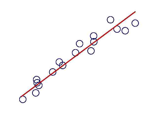
На практике вид функции чаще всего определяют путем сравнения расположения точек с графиками известных функций.

Полученная формула y=F(x), которую называют эмпирической формулой, или уравнением регрессии y на x, или приближающей (аппроксимирующей) функцией, позволяет находить значения f(x) для нетабличных значений x, сглаживая результаты измерений величины y.

Для того, чтобы получить параметры функции F, используется метод наименьших квадратов. В этом методе в качестве критерия близости приближающей функции к совокупности точек используется суммы квадратов разностей значений табличных значений y и теоретических, рассчитанных по уравнению регрессии.

Таким образом, нам требуется найти функцию F, такую, чтобы сумма квадратов S была наименьшей:

Рассмотрим решение этой задачи на примере получения линейной регрессии F=ax+b.
S является функцией двух переменных, a и b. Чтобы найти ее минимум, используем условие экстремума, а именно, равенства нулю частных производных.

Используя формулу производной сложной функции, получим следующую систему уравнений:
$begin{cases} sum [y_i - F(x_i, a, b)]cdot F^prime_a(x_i, a, b)=0 \ sum [y_i - F(x_i, a, b)]cdot F^prime_b(x_i, a, b)=0 end{cases}$

Для функции вида частные производные равны:
,

Подставив производные, получим:
$begin{cases} sum (y_i - ax_i-b)cdot x_i=0 \ sum (y_i - ax_i-b)=0 end{cases}$

Далее:
$begin{cases} sum y_ix_i - a sum x_i^2-bsum x_i=0 \ sum y_i - asum x_i - nb=0 end{cases}$

Откуда, выразив a и b, можно получить формулы для коэффициентов линейной регрессии, приведенные выше.
Аналогичным образом выводятся формулы для остальных видов регрессий.

Источник

Quadratic regression is a type of a multiple linear regression. It can be manually found by using the least squares method. Use our online quadratic regression calculator to find the quadratic regression equation with graph.

Find the Quadratic Regression Equation with Graph

Code to add this calci to your website

Formula:

Quadratic Regression Equation(y) = a + b x + c x^2
c = { [ Σ x² y * Σ xx ] – [Σ xy * Σ xx² ] } / { [ Σ xx * Σ x²x ²] – [Σ xx² ]² }
b = { [ Σ xy * Σ x²x² ] – [Σ x²y * Σ xx² ] } / { [ Σ xx * Σ x²x ²] – [Σ xx² ]² }
a = [ Σ y / n ] – { b * [ Σ x / n ] } – { a * [ Σ x ² / n ] }

Where ,

Σ x x = [ Σ x ² ] – [ ( Σ x )² / n ]
Σ x y = [ Σ x y ] – [ ( Σ x * Σ y ) / n ]
Σ x x² = [ Σ x ³ ] – [ ( Σ x ² * Σ x ) / n ]
Σ x² y = [ Σ x ² y] – [ ( Σ x ² * Σ y ) / n ]
Σ x² x² = [ Σ x ⁴ ] – [ ( Σ x ² )² / n ]
x and y are the Variables.
a, b, and c are the Coefficients of the Quadratic Equation
n = Number of Values or Elements
Σ x= Sum of First Scores
Σ y = Sum of Second Scores
Σ x²= Sum of square of First Scores
Σ x³= Sum of Cube of First Scores
Σ x⁴ = Sum of Power Four of First Scores
Σ xy= Sum of the Product of First and Second Scores
Σ x²y = Sum of Square of First Scores and Second Scores

Quadratic Regression is a process of finding the equation of parabola that best suits the set of data. The equation can be defined in the form as a x² + b x + c. Quadratic regression is an extension of simple linear regression. While linear regression can be performed with as few as two points, whereas quadratic regression can only be performed with more data points to be certain your data falls into the “U” shape. Just enter the set of X and Y values separated by comma in the given quadratic regression calculator to get the best fit second degree quadratic regression and graph.

All the results including graphs generated by this quadratic regression calculator are accurate. Make use of this quadratic regression equation calculator to do the statistics calculation in simple with ease.

Related Calculators:

Linear Regression Calculator
Correlation Coefficient Calculator
Autocorrelation Calculator
Regression Coefficient Confidence Interval
Spearman’s Rank Correlation Coefficient (RHO) Calculator
Golf Handicap Calculator
Central Limit Theorem Calculator (CLT)

Источник

Линейная регрессия это способ описания зависимости между двумя или более исходными данными. При использовании линейная регрессии в математическом анализе можно узнать:
Зависимость одной переменной (y) от переменной(x), или нескольких других переменных.
На сколько значение (y) может изменяться в зависимости от значения (x).
На сколько значение (y) зависит от значения (x).
Появляется возможность предсказать значение (y) от значения (x).

Калькулятор расчета регрессии

Важно! В качестве разделителя для чисел используйте пробел

Значение Y (зависимая переменная от x)

Значение X (независимая переменная или предиктор)

Корреляция или R² (свидетельствует о том, что между двумя числовыми диапазонами существует сильная прямая взаимосвязь. Возможные значения от -1 до +1, если 0 то переменные не зависят друг от друга.)

Наклон (величина, на которую Y увеличивается в среднем, если мы увеличиваем X на одну единицу)

Пересечение или Intercept (это значение Y, когда X=0 )

Предсказать значение Y при помощи линейной регрессии

Введите X (для определения Y)

Значение Y (в зависимости от X будет равно)

Формулы

Уравнение регрессии Y = a + bx
Наклон b = (NΣXY — (ΣX)(ΣY)) / (NΣX² — (ΣX)²)
Перехват a = (ΣY — b(ΣX)) / N
a = Точка пересечения линии регрессии и оси y
b = Наклон линии регрессии
X и Y-переменные
N = Количество значений или элементов

Как пользоваться калькулятором линейной регрессии

Самый простой способ понять что такое линейная регрессия, это объяснить все на конкретном примере.

За исходными данными обратимся к официальному сайту федеральной службы государственной статистики. Возьмем от туда размер средней пенсии в России за последние одиннадцать лет и введем эти числа в поле Y, (15400 14900 14300 13620 13132 11783 10888 10400 9040 8202 7476 5191). Теперь в поле X внесем соответствующие им года (2020 2019 2018 2017 2016 2015 2014 2013 2012 2011 2010 2009).

После нажатия на кнопку «Вычислить», в поле «Наклон» (взято математическое название данной величины, не сарказм), вы увидите величину на которую каждый год изменяется размер средней пенсии. Поле «Корреляция» говорит нам о том, на сколько эти два числовых диапазона взаимосвязаны. Если ближе к -1, то противоположная связь. Если ближе к +1, то значение Y прямо зависит от значения X. Ели ближе к нулю, то зависимость между данными отсутствует.

Если вы хотите предсказать какое нибудь значение, тогда воспользуйтесь второй частью данного калькулятора. В поле «Введите X» поставьте год, в котором вы хотите узнать какой будет размер пенсии, затем нажмите «Вычислить». В поле «Значение Y» появится число, означающее размер пенсии в соответствующий период времени. Например если в поле «Введите X» поставим 2024 год, то узнаем какая средняя пенсия будет в этом году, она равна 19624 рублей.

Источник

Instructions:

Perform a regression analysis by using the

Linear Regression Calculator

, where the regression equation will be found and a detailed report of the calculations will be provided,
along with a scatter plot. All you have to do is type your X and Y data. Optionally, you can add a title and add the name of the variables.

More about this Linear Regression Calculator

linear regression model

corresponds to a linear model that minimizes the sum of squared errors for a set of pairs ((X_i, Y_i)).

This is, you assume the existence of a model which in its simplified form is (Y = alpha + beta X) and then you take note of
the discrepancies (errors) found when using this linear model to predict the set of given data.

For each (X_i) in the data, you compute (hat Y_i = alpha + beta X_i), and you compute the error by measuring (Y_i – hat Y_i).
More specifically, in this case you take the square of each discrepancy/error and you add up ALL these square errors.

The objective of a regression calculator is to find the best values of (alpha) and (beta) so that the sum of squared errors is
as small as possible.

Regression Formula

The linear regression equation, also known as least squares equation has the following form: (hat Y = a + b X), where the
regression coefficients are the values of (a) and (b).

The question is: How to calculate the regression coefficients? The regression coefficients are computed by this regression calculator as follows:

[b = frac{SS_{XY}}{SS_{XX}}]
[a = bar Y – bar X cdot b ]

These are the formulas you used if you were to calculate the regression equation by hand, but likely you will prefer to use
a calculator (our regression calculator) which will show you the important steps.

This linear regression formula is interpreted as follows: The coefficient (b) is known as the slope coefficient, and
the coefficient (a) is known as the y-intercept.

If instead of a linear model, you would like to use a non-linear model, then you should consider instead a

polynomial regression calculator

, which allows you to use powers of the independent variable.

Linear regression calculator Steps

First of all, you want to assess whether or not it makes sense to run a regression analysis. So then first you
should run this correlation coefficient calculator to see if there is a
significant degree of linear association between the the variables.

In other words, it only makes sense to run a regression analysis the correlation coefficient is strong enough to make a
case for a linear regression model. Also, you should use this scatter plot calculator to ensure that the visual
pattern is indeed linear.

It is conceivable that a correlation coefficient is close to 1, but yet the pattern of association is not linear at all.

The steps to conduct a regression analysis are:

Step 1: Get the data for the dependent and independent variable in column format.

Step 2: Type in the data or you can paste it if you already have in Excel format for example.

Step 3: Press “Calculate”.

This regression equation calculator with steps will provide you with all the calculations required, in an organized manner, so
that you can clearly understand all the steps of the process.

Regression Residuals

How do we assess if a linear regression model is good? You may think “easy, just look at the

scatterplot

“. In reality, math and statistics tend to go beyond where the eye meets the graph.
It is usually risky to rely solely on the scatterplot to assess the quality of the model.

In terms of goodness of fit, one way of assessing the quality of fit of a linear regression model is by

computing the coefficient of determination

, indicates the proportion of variation that in the dependent variable that is explained by the independent variable.

In linear regression, the fulfillment of the assumptions is crucial so that the estimates of the regression coefficient
have good properties (being unbiased, minimum variance, among others).

In order to asses the linear regression assumptions, you will need to take a look at the residuals. For that purpose,
you can take a look at our

residual calculator

Predictive Power of a Regression Equation

How can you tell if the regression equation found is good? Or a better question, how to know whether or not the regression equation
estimated has good predictive power?

What you need to do is to compute the coefficient of determination, which tells you
the amount of variation in the dependent variable that is explained by the dependent variable(s).

For a simple regression model (with one independent variable), the coefficient of determination is simply computed by squaring the
correlation coefficient.

For example, if the correlation coefficient is r = 0.8, then the coefficient of
determination is (r^2 = 0.8^2 = 0.64) and the
interpretation is that 64% of the variation in the dependent variable are explained by the independent variable in this model.

Polynomial regression

As we have mentioned before, there are times where the linear regression is simply not appropriate, because there is a clear non-liner pattern governing the
relationship between two variables.

Your first signal that polynomial regression should be used instead of linear regression is to see that there is a curvilinear pattern in
the data presented by the scatterplot.

If that is the case, you could try this polynomial regression calculator, to estimate a non-linear
model that has a better chance of having a better fit.

What is given by this online linear regression calculator?

First, you get a tabulation of the data, and you calculate the corresponding squares and cross-multiplications to get the required
sum of squared values, needed to apply the regression formula.

Once that is all neatly shown in a table with all the needed columns, the regression formulas will be shown, with the correct values
being plugged in and then with a conclusion about the linear regression model that was estimated from the data.

Also, a scatter plot is constructed in order to assess how tight the linear association is between the variables, which gives an indication
of how good the linear regression model is.

Is r2 the regression coefficient?

No. Technically, the regression coefficients are the coefficients estimated that are part of the regression model. The r2 coefficient
is called the coefficient of determination.

The coefficient r2 is also computed from sample data, but it is not a regression coefficient, but it does not mean it is not important.
The r2 coefficient is important because it gives an estimation of the percentage of variation explained by the model.

How to do linear regression in Excel?

Excel has the ability of conducting linear regression by either directly using the commands “=SLOPE()” and “=INTERCEPT()”, or by using
the Data Analysis menu.

But Excel does not show all the steps like our regression calculator does.

Other calculators related to linear regression

This regression equation calculator is only one among many calculators of interest when dealing with linear models.
You may also be interested in

computing the correlation coefficient

, or to

construct a scatter plot

with the data provided.

What is the coefficient of determination?

The coefficient of determination, or R^2 is a measurement of the proportion of the variation in the dependent variable that
is explained by the independent variable.

For example, assume that we have a coefficient of determination of R^2 = 0.67 when estimating a linear regression of Y
as a function of X, then the interpretation is that X explains 67% of the variation in Y.

What happens when you have more variables

You could potentially have more than one independent variable. For example, you may be interested in estimating Y in terms
of two variables X1 and X2. In that case, you need to
calculate a multiple linear regression model, where the idea is essentially
the same: find the hyperplane that minimize the sum of squared errors.

Источник

МНК и регрессионный анализ Онлайн + графики

Аппроксимация функции одной переменной

Линейная регрессия

Квадратичная регрессия

Кубическая регрессия

Степенная регрессия

Показательная регрессия

Гиперболическая регрессия

Логарифмическая регрессия

Экспоненциальная регрессия

Вывод формул

Find the Quadratic Regression Equation with Graph

Formula:

Where ,

Related Calculators:

Формулы

Как пользоваться калькулятором линейной регрессии

More about this Linear Regression Calculator

Regression Formula

Linear regression calculator Steps

Regression Residuals

Predictive Power of a Regression Equation

Polynomial regression

What is given by this online linear regression calculator?

Is r2 the regression coefficient?

How to do linear regression in Excel?

Other calculators related to linear regression

What is the coefficient of determination?

What happens when you have more variables

Вам также может понравиться

Как составить правильное питание в пост

Как составить письмо с описью для налоговой

Как найти компьютер по имени в домене

Добавить комментарий Отменить ответ