Как найти значение биномиальных коэффициентов - Сайт, где вы сможете решить свои вопросы

Биномиальный коэффициент — коэффициент перед членом разложения бинома Ньютона $(1+x)^{n}$ по степеням . Коэффициент при $x^{k}$ обозначается или и читается «биномиальный коэффициент из по » (или «число сочетаний из по »):

${displaystyle (1+x)^{n}={binom {n}{0}}+{binom {n}{1}}x+{binom {n}{2}}x^{2}+ldots +{binom {n}{n}}x^{n}=sum _{k=0}^{n}{binom {n}{k}}x^{k}}$

для натуральных степеней .

Биномиальные коэффициенты могут быть также определены для произвольных действительных показателей . В случае произвольного действительного числа биномиальные коэффициенты определяются как коэффициенты разложения выражения $(1+x)^{n}$ в бесконечный степенной ряд:

${displaystyle (1+x)^{n}=sum _{k=0}^{infty }{binom {n}{k}}x^{k}}$

где в случае неотрицательных целых все коэффициенты при k>n обращаются в нуль и поэтому данное разложение является конечной суммой.

В комбинаторике биномиальный коэффициент для неотрицательных целых чисел и интерпретируется как количество сочетаний из по , то есть как количество всех (нестрогих) подмножеств (выборок) размера в -элементном множестве.

Биномиальные коэффициенты часто возникают в задачах комбинаторики и теории вероятностей. Обобщением биномиальных коэффициентов являются мультиномиальные коэффициенты.

Явные формулы[править | править код]

Вычисляя коэффициенты в разложении $(1+x)^{n}$ в степенной ряд, можно получить явные формулы для биномиальных коэффициентов .

Для всех действительных чисел и целых чисел :

${displaystyle {binom {n}{k}}={begin{cases}{frac {n(n-1)(n-2)cdot ldots cdot (n-k+1)}{k!}},&kgeqslant 0\0,&k<0end{cases}}}$

где обозначает факториал числа .

Для неотрицательных целых и также справедливы формулы:

${displaystyle {binom {n}{k}}={begin{cases}{frac {n!}{k!(n-k)!}},&0leqslant kleqslant n\0,&k>nend{cases}}}$

Для целых отрицательных показателей коэффициенты разложения бинома ${displaystyle (1+x)^{-n}}$ равны:

${displaystyle {binom {-n}{k}}={begin{cases}(-1)^{k}cdot {frac {(n+k-1)!}{k!(n-1)!}},&kgeqslant 0\0,&k<0end{cases}}}$

Треугольник Паскаля[править | править код]

Визуализация биномиального коэффициента до 4 степени

Тождество:

{n choose k}={n-1 choose k-1}+{n-1 choose k}

позволяет расположить биномиальные коэффициенты для неотрицательных целых чисел , в виде треугольника Паскаля, в котором каждое число равно сумме двух вышестоящих:

${begin{matrix}n=0:&&&&&1&&&&\n=1:&&&&1&&1&&&\n=2:&&&1&&2&&1&&\n=3:&&1&&3&&3&&1&\n=4:&1&&4&&6&&4&&1\vdots &&vdots &&vdots &&vdots &&vdots &end{matrix}}$

Треугольная таблица, предложенная Паскалем в «Трактате об арифметическом треугольнике» (1654), отличается от той, что выписана здесь, поворотом на 45°. Таблицы для изображения биномиальных коэффициентов были известны и ранее (Тарталье, Омару Хайяму).

Если в каждой строке треугольника Паскаля все числа разделить на $2^{n}$ (это сумма всех чисел в строке), то все строки при стремлении к бесконечности примут вид функции нормального распределения.

Свойства[править | править код]

Производящие функции[править | править код]

Для фиксированного значения производящей функцией последовательности биномиальных коэффициентов является:

${displaystyle sum _{k=0}^{infty }{binom {n}{k}}x^{k}=(1+x)^{n}}$

Для фиксированного значения производящая функция последовательности коэффициентов равна:

${displaystyle sum _{n}{binom {n}{k}}y^{n}={frac {y^{k}}{(1-y)^{k+1}}}}$

Двумерной производящей функцией биномиальных коэффициентов для целых n,k является:

${displaystyle sum _{n,k}{binom {n}{k}}x^{k}y^{n}={frac {1}{1-y-xy}}}$

, или ${displaystyle sum _{n=0}^{infty }sum _{k=0}^{n}{binom {n}{k}}x^{k}y^{n}={frac {1}{1-y-xy}}}$

Делимость[править | править код]

Из теоремы Люка следует, что:

Основные тождества[править | править код]

.
${displaystyle {binom {n}{k}}=(-1)^{k}{binom {-n+k-1}{k}}}$ .
(правило симметрии).
${displaystyle {n choose k}={frac {n}{k}}{n-1 choose k-1}}$ (вынесение за скобки).
(замена индексов).
.

Бином Ньютона и следствия[править | править код]

а более общем виде

${displaystyle sum _{k=-a}^{a}(-1)^{k}{a+b choose a+k}{b+c choose b+k}{c+a choose c+k}={frac {(a+b+c)!}{a!,b!,c!}}}$

Свёртка Вандермонда и следствия[править | править код]

Свёртка Вандермонда:

${displaystyle sum _{k}{r choose m+k}{s choose n-k}={r+s choose m+n}}$

где а . Это тождество получается вычислением коэффициента при ${displaystyle x^{m+n}}$ в разложении ${displaystyle (1+x)^{r}(1+x)^{s}}$ с учётом тождества ${displaystyle (1+x)^{r+s}=(1+x)^{r}(1+x)^{s}}$ . Сумма берётся по всем целым , для которых . Для произвольных действительных , число ненулевых слагаемых в сумме будет конечно.

Следствие свёртки Вандермонда:

${n choose 0}{a choose a}-{n choose 1}{a+1 choose a}+ldots +(-1)^{n}{n choose n}{a+n choose a}=(-1)^{n}{a choose n}$

Более общее тождество:

$sum _{{i=0}}^{{p}}(-1)^{i}{p choose i}prod _{{m=1}}^{{n}}{i+s_{m} choose s_{m}}=0$

, если $sum _{{m=1}}^{n}{s_{m}}<p$

Ещё одним следствием свёртки является следующее тождество:
${displaystyle {n choose 0}^{2}+{n choose 1}^{2}+ldots +{n choose n}^{2}={2n choose n}}$ .

Другие тождества[править | править код]

${displaystyle {binom {n}{t}}+{binom {n}{t+s}}+{binom {n}{t+2s}}+ldots ={frac {1}{s}}sum _{j=0}^{s-1}left(2cos {frac {pi j}{s}}right)^{n}cos {frac {pi (n-2t)j}{s}}}$

Также имеют место равенства:

${displaystyle {begin{alignedat}{2}{binom {n}{3}}&={frac {n(n-1)(n-2)}{color {Green}2}}-sum _{i=2}^{n-1}{(n-i)(n-i+1)}=\&=n(n-1)(n-2)-sum _{i=2}^{n-1}{(n-i)({color {Green}2}n-i+1)}=\&=3{binom {n}{3}}-2{binom {n}{3}};\end{alignedat}}}$

${displaystyle {begin{alignedat}{2}{binom {n}{4}}&={frac {n(n-1)(n-2)(n-3)}{color {Green}2}}-sum _{i=3}^{n-1}{(n-i)left(n(n-1)-sum _{i_{0}=1}^{i-2}i_{0}right)}=\&=n(n-1)(n-2)(n-3)-sum _{i=3}^{n-1}{(n-i)left({color {Green}2}n(n-1)-sum _{i_{0}=1}^{i-2}i_{0}right)}=\&=24{binom {n}{4}}-23{binom {n}{4}};\end{alignedat}}}$

${displaystyle {begin{alignedat}{2}{binom {n}{5}}&={frac {n(n-1)(n-2)(n-3)(n-4)}{color {Green}2}}-\&-sum _{i=4}^{n-1}{(n-i)left(n(n-1)(n-2)-sum _{i_{0}=1}^{i-3}sum _{i_{1}=1}^{i_{0}}i_{1}right)}=\&=n(n-1)(n-2)(n-3)(n-4)-\&-sum _{i=4}^{n-1}{(n-i)left({color {Green}2}n(n-1)(n-2)-sum _{i_{0}=1}^{i-3}sum _{i_{1}=1}^{i_{0}}i_{1}right)}=\&=120{binom {n}{5}}-119{binom {n}{5}}.end{alignedat}}}$

Откуда следует:

${displaystyle {binom {n}{3}}={frac {sum limits _{i=2}^{n-1}{(n-i)(2n-i+1)}}{2}}={frac {sum limits _{i=2}^{n-1}{(n-i)left(2A_{n}^{1}-{binom {i-1}{1}}right)}}{2}};}$

${displaystyle {binom {n}{4}}={frac {sum limits _{i=3}^{n-1}{(n-i)left(2n(n-1)-sum limits _{i_{0}=1}^{i-2}i_{0}right)}}{23}}={frac {sum limits _{i=3}^{n-1}{(n-i)left(2A_{n}^{2}-{binom {i-1}{2}}right)}}{23}};}$

${displaystyle {begin{alignedat}{2}&{binom {n}{5}}={frac {sum limits _{i=4}^{n-1}{(n-i)left(2n(n-1)(n-2)-sum limits _{i_{0}=1}^{i-3}sum limits _{i_{1}=1}^{i_{0}}i_{1}right)}}{119}}=\&={frac {sum limits _{i=4}^{n-1}{(n-i)left(2A_{n}^{3}-{binom {i-1}{3}}right)}}{119}};\end{alignedat}}}$

${displaystyle {binom {n}{k}}={frac {sum limits _{i=k-1}^{n-1}{(n-i)left(2A_{n}^{k-2}-{binom {i-1}{k-2}}right)}}{k!-1}}}$

где $A_{n}^{k}$ — количество размещений из по .

Матричные соотношения[править | править код]

Если взять квадратную матрицу, отсчитав элементов по катетам треугольника Паскаля и повернув матрицу на любой из четырёх углов, то детерминант этих четырёх матриц равен ±1 при любом , причём детерминант матрицы с вершиной треугольника в верхнем левом углу равен 1.

В матрице числа на диагонали повторяют числа строк треугольника Паскаля (). Её можно разложить в произведение двух строго диагональных матриц: нижнетреугольной и получаемой из неё транспонированием:

${displaystyle {begin{bmatrix}{binom {i+j}{i}}end{bmatrix}}=UU^{T}}$

где . Обратная матрица к имеет вид:

${displaystyle U^{-1}={begin{bmatrix}(-1)^{i+j}{binom {i}{j}}end{bmatrix}}}$

Таким образом, можно разложить обратную матрицу к в произведение двух строго диагональных матриц: первая матрица — верхнетреугольная, а вторая получается из первой путём транспонирования, что позволяет дать явное выражение для обратных элементов:

${begin{bmatrix}{binom {i+j}{i}}end{bmatrix}}_{{m,n}}^{{-1}}=sum _{{k=0}}^{{p}}(-1)^{{m+n}}{binom {k}{m}}{binom {k}{n}}$

, где

Элементы обратной матрицы меняются при изменении её размера и, в отличие от матрицы , недостаточно приписать новую строку и столбец. Столбец матрицы есть многочлен степени по аргументу , следовательно, первые p столбцов образуют полный базис в пространстве векторов длины +1, чьи координаты могут быть интерполированы многочленом равной или меньшей степени p-1 . Нижняя строка матрицы ${begin{bmatrix}{binom {i+j}{i}}end{bmatrix}}_{{m,n}}^{{-1}}$ ортогональна любому такому вектору.

${begin{bmatrix}{binom {i+j}{i}}end{bmatrix}}_{{p,n}}^{{-1}}=sum _{{k=0}}^{{p}}(-1)^{{p+n}}{binom {k}{p}}{binom {k}{n}}=(-1)^{{p+n}}{binom {p}{n}}$

$sum _{{n=0}}^{{p}}(-1)^{{p+n}}{binom {p}{n}}{P}_{{a}}(n)=0$

при

, где ${P}_{{a}}(n)$

многочлен степени

Если произвольный вектор длины p+1 можно интерполировать многочленом степени i<p , то скалярное произведение со строками (нумерация с 0) матрицы ${begin{bmatrix}{binom {i+j}{i}}end{bmatrix}}_{{m,n}}^{{-1}}$ равно нулю.
Используя тождество выше и равенство единицы скалярного произведения нижней строки матрицы ${begin{bmatrix}{binom {i+j}{i}}end{bmatrix}}_{{m,n}}^{{-1}}$ на последний столбец матрицы , получаем:

${displaystyle sum _{n=0}^{p}(-1)^{p+n}{binom {p}{n}}{n}^{p}=p!}$

Для показателя большего можно задать рекуррентную формулу:

${displaystyle sum _{n=0}^{p}(-1)^{p+n}{binom {p}{n}}{n}^{p+a}=p!{P}_{2a}(p)={f}_{a}(p)}$

где многочлен

${displaystyle {P}_{2a+2}(p)=sum _{x=1}^{p}x{P}_{2a}(x);quad ageqslant 0;quad {P}_{0}(p)=1}$

Для доказательства сперва устанавливается тождество:

${displaystyle {f}_{a}(p+1)=sum _{x=0}^{a}{(p+1)}^{x+1}{f}_{a-x}(p)}$

Если требуется найти формулу не для всех показателей степени, то:

${displaystyle {P}_{2a}(p)={frac {p}{{2}^{a}}}{binom {p+a}{a}}{Q}_{a-1}(p);quad a>0}$

Старший коэффициент ${Q}_{{a-1}}(p)$ равен 1, потребуется a-1 значений, чтобы найти другие коэффициенты:

${Q}_{{a-1}}(p)=p(p+1){T}_{{a-3}}(p)$

для

{displaystyle aequiv 1{pmod {2}};ageqslant 3}

Асимптотика и оценки[править | править код]

Непосредственно из формулы Стирлинга следует, что для верно $C_{n}^{{alpha n}}sim {sqrt {{frac {1}{2pi alpha (1-alpha )n}}}}left({{frac {1}{alpha }}}right)^{{alpha n}}left({{frac {1}{1-alpha }}}right)^{{(1-alpha )n}}=left({{frac {1}{alpha ^{alpha }{(1-alpha )}^{{(1-alpha )}}}}+o(1)}right)^{{n}}$ .

Целозначные полиномы[править | править код]

Биномиальные коэффициенты ${displaystyle {tbinom {x}{0}}=1,{tbinom {x}{1}}=x,{tbinom {x}{2}}={tfrac {x^{2}}{2}}-{tfrac {x}{2}}}$ , … являются целозначными полиномами от , то есть принимают целые значения при целых значениях , — это нетрудно понять, например, по треугольнику Паскаля. Более того, они образуют базис целозначных полиномов, в котором все целозначные полиномы выражаются как линейные комбинации с целыми коэффициентами.^[1]

В то же время стандартный базис ${displaystyle 1,x,x^{2}}$ , … не позволяет выразить все целочисленные полиномы, если использовать только целые коэффициенты, так как уже ${displaystyle {tbinom {x}{2}}={tfrac {x^{2}}{2}}-{tfrac {x}{2}}}$ имеет дробные коэффициенты при степенях .

Этот результат обобщается на полиномы многих переменных. А именно, если полином степени имеет вещественные коэффициенты и принимает целые значения при целых значениях переменных, то

${displaystyle R(x_{1},dots ,x_{m})=Pleft({binom {x_{1}}{1}},dots ,{binom {x_{1}}{k}},dots ,{binom {x_{m}}{1}},dots ,{binom {x_{m}}{k}}right)}$

где — полином с целыми коэффициентами.^[2]

Алгоритмы вычисления[править | править код]

Биномиальные коэффициенты можно вычислить с помощью рекуррентной формулы , если на каждом шаге хранить значения при . Этот алгоритм особенно эффективен, если нужно получить все значения при фиксированном . Алгоритм требует O(n) памяти ( $O(n^{2})$ при вычислении всей таблицы биномиальных коэффициентов) и $O(n^{2})$ времени (в предположении, что каждое число занимает единицу памяти и операции с числами выполняются за единицу времени), где — «» большое.

При фиксированном значении биномиальные коэффициенты могут быть вычислены по рекуррентной формуле ${displaystyle {tbinom {n}{k}}={tfrac {n}{n-k}}cdot {tbinom {n-1}{k}}}$ с начальным значением . Для вычисления значения этот метод требует O(1) памяти и O(n) времени.

Если требуется вычислить коэффициенты при фиксированном значении , можно воспользоваться формулой ${displaystyle {tbinom {n}{k}}={tfrac {n-k+1}{k}}cdot {tbinom {n}{k-1}}}$ при начальном условии . При каждом шаге итерации числитель уменьшается на (начальное значение равно ), а знаменатель соответственно увеличивается на (начальное значение — ). Для вычисления значения этот метод требует O(1) памяти и O(k) времени.

Примечания[править | править код]

↑ Прасолов В. В. Глава 12. Целозначные многочлены // Многочлены. — М.: МЦНМО, 1999, 2001, 2003. Архивная копия от 21 января 2022 на Wayback Machine
↑ Ю. Матиясевич. Десятая проблема Гильберта. — Наука, 1993.

Литература[править | править код]

Биномиальные коэффициенты // Энциклопедический словарь Брокгауза и Ефрона : в 86 т. (82 т. и 4 доп.). — СПб., 1890—1907.
Фукс Д., Фукс М. Арифметика биномиальных коэффициентов // Квант. — 1970. — № 6. — С. 17—25.
Кузьмин О. В. Треугольник и пирамида Паскаля: свойства и обобщения // Соросовский Образовательный Журнал. — 2000. — Т. 6, № 5. — С. 101—109.
Ландо С. К. Теневое исчисление // VIII летняя школа «Современная математика». — Дубна, 2008.
Винберг Э. Б. Удивительные арифметические свойства биномиальных коэффициентов // Математическое просвещение. — 2008. — Вып. 12. — С. 33–42.
Дональд Кнут, Роналд Грэхем, Орен Паташник. Конкретная математика. Математические основы информатики = Concrete Mathematics. A Foundation for Computer Science. — 2-е. — М.: Мир; Бином. Лаборатория знаний; «Вильямс», 1998—2009. — 703, 784 с. — ISBN 95-94774-560-7, 78-5-8459-1588-7.

Источник

The binomial coefficients can be arranged to form Pascal’s triangle, in which each entry is the sum of the two immediately above.

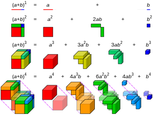
Visualisation of binomial expansion up to the 4th power

In mathematics, the binomial coefficients are the positive integers that occur as coefficients in the binomial theorem. Commonly, a binomial coefficient is indexed by a pair of integers n ≥ k ≥ 0 and is written It is the coefficient of the x^k term in the polynomial expansion of the binomial power (1 + x)ⁿ; this coefficient can be computed by the multiplicative formula

${displaystyle {binom {n}{k}}={frac {ntimes (n-1)times cdots times (n-k+1)}{ktimes (k-1)times cdots times 1}},}$

which using factorial notation can be compactly expressed as

${displaystyle {binom {n}{k}}={frac {n!}{k!(n-k)!}}.}$

For example, the fourth power of 1 + x is

${displaystyle {begin{aligned}(1+x)^{4}&={tbinom {4}{0}}x^{0}+{tbinom {4}{1}}x^{1}+{tbinom {4}{2}}x^{2}+{tbinom {4}{3}}x^{3}+{tbinom {4}{4}}x^{4}\&=1+4x+6x^{2}+4x^{3}+x^{4},end{aligned}}}$

and the binomial coefficient ${displaystyle {tbinom {4}{2}}={tfrac {4times 3}{2times 1}}={tfrac {4!}{2!2!}}=6}$ is the coefficient of the x² term.

Arranging the numbers in successive rows for gives a triangular array called Pascal’s triangle, satisfying the recurrence relation

{displaystyle {binom {n}{k}}={binom {n-1}{k-1}}+{binom {n-1}{k}}.}

The binomial coefficients occur in many areas of mathematics, and especially in combinatorics. The symbol is usually read as “n choose k” because there are ways to choose an (unordered) subset of k elements from a fixed set of n elements. For example, there are ways to choose 2 elements from namely and

The binomial coefficients can be generalized to for any complex number z and integer k ≥ 0, and many of their properties continue to hold in this more general form.

History and notation[edit]

Andreas von Ettingshausen introduced the notation in 1826,^[1] although the numbers were known centuries earlier (see Pascal’s triangle). In about 1150, the Indian mathematician Bhaskaracharya gave an exposition of binomial coefficients in his book Līlāvatī.^[2]

Alternative notations include C(n, k), _nC_k, ⁿC_k, C^k_n, Cⁿ_k, and C_n,k in all of which the C stands for combinations or choices. Many calculators use variants of the C notation because they can represent it on a single-line display. In this form the binomial coefficients are easily compared to k-permutations of n, written as P(n, k), etc.

Definition and interpretations[edit]

k n	0	1	2	3	4	⋯
0	1	0	0	0	0	⋯
1	1	1	0	0	0	⋯
2	1	2	1	0	0	⋯
3	1	3	3	1	0	⋯
4	1	4	6	4	1	⋯
⋮	⋮	⋮	⋮	⋮	⋮	⋱
The first few binomial coefficients on a left-aligned Pascal’s triangle

For natural numbers (taken to include 0) n and k, the binomial coefficient can be defined as the coefficient of the monomial X^k in the expansion of (1 + X)ⁿ. The same coefficient also occurs (if k ≤ n) in the binomial formula

$(x+y)^{n}=sum _{k=0}^{n}{binom {n}{k}}x^{n-k}y^{k}$

(∗)

(valid for any elements x, y of a commutative ring),
which explains the name “binomial coefficient”.

Another occurrence of this number is in combinatorics, where it gives the number of ways, disregarding order, that k objects can be chosen from among n objects; more formally, the number of k-element subsets (or k-combinations) of an n-element set. This number can be seen as equal to the one of the first definition, independently of any of the formulas below to compute it: if in each of the n factors of the power (1 + X)ⁿ one temporarily labels the term X with an index i (running from 1 to n), then each subset of k indices gives after expansion a contribution X^k, and the coefficient of that monomial in the result will be the number of such subsets. This shows in particular that is a natural number for any natural numbers n and k. There are many other combinatorial interpretations of binomial coefficients (counting problems for which the answer is given by a binomial coefficient expression), for instance the number of words formed of n bits (digits 0 or 1) whose sum is k is given by , while the number of ways to write ${displaystyle k=a_{1}+a_{2}+cdots +a_{n}}$ where every a_i is a nonnegative integer is given by . Most of these interpretations are easily seen to be equivalent to counting k-combinations.

Computing the value of binomial coefficients[edit]

Recursive formula[edit]

One method uses the recursive, purely additive formula

for all integers n,k such that

with initial/boundary values

for all integers

The formula follows from considering the set {1, 2, 3, …, n} and counting separately (a) the k-element groupings that include a particular set element, say “i“, in every group (since “i” is already chosen to fill one spot in every group, we need only choose k − 1 from the remaining n − 1) and (b) all the k-groupings that don’t include “i“; this enumerates all the possible k-combinations of n elements. It also follows from tracing the contributions to X^k in (1 + X)ⁿ⁻¹(1 + X). As there is zero Xⁿ⁺¹ or X⁻¹ in (1 + X)ⁿ, one might extend the definition beyond the above boundaries to include when either k > n or k < 0. This recursive formula then allows the construction of Pascal’s triangle, surrounded by white spaces where the zeros, or the trivial coefficients, would be.

Multiplicative formula[edit]

A more efficient method to compute individual binomial coefficients is given by the formula

${displaystyle {binom {n}{k}}={frac {n^{underline {k}}}{k!}}={frac {n(n-1)(n-2)cdots (n-(k-1))}{k(k-1)(k-2)cdots 1}}=prod _{i=1}^{k}{frac {n+1-i}{i}},}$

where the numerator of the first fraction $n^{underline {k}}$ is expressed as a falling factorial power.
This formula is easiest to understand for the combinatorial interpretation of binomial coefficients.
The numerator gives the number of ways to select a sequence of k distinct objects, retaining the order of selection, from a set of n objects. The denominator counts the number of distinct sequences that define the same k-combination when order is disregarded.

Due to the symmetry of the binomial coefficient with regard to k and n − k, calculation may be optimised by setting the upper limit of the product above to the smaller of k and n − k.

Factorial formula[edit]

Finally, though computationally unsuitable, there is the compact form, often used in proofs and derivations, which makes repeated use of the familiar factorial function:

${displaystyle {binom {n}{k}}={frac {n!}{k!,(n-k)!}}quad {text{for }} 0leq kleq n,}$

where n! denotes the factorial of n. This formula follows from the multiplicative formula above by multiplying numerator and denominator by (n − k)!; as a consequence it involves many factors common to numerator and denominator. It is less practical for explicit computation (in the case that k is small and n is large) unless common factors are first cancelled (in particular since factorial values grow very rapidly). The formula does exhibit a symmetry that is less evident from the multiplicative formula (though it is from the definitions)

(1)

which leads to a more efficient multiplicative computational routine. Using the falling factorial notation,

${displaystyle {binom {n}{k}}={begin{cases}n^{underline {k}}/k!&{text{if }} kleq {frac {n}{2}}\n^{underline {n-k}}/(n-k)!&{text{if }} k>{frac {n}{2}}end{cases}}.}$

Generalization and connection to the binomial series[edit]

The multiplicative formula allows the definition of binomial coefficients to be extended^[3] by replacing n by an arbitrary number α (negative, real, complex) or even an element of any commutative ring in which all positive integers are invertible:

${displaystyle {binom {alpha }{k}}={frac {alpha ^{underline {k}}}{k!}}={frac {alpha (alpha -1)(alpha -2)cdots (alpha -k+1)}{k(k-1)(k-2)cdots 1}}quad {text{for }}kin mathbb {N} {text{ and arbitrary }}alpha .}$

With this definition one has a generalization of the binomial formula (with one of the variables set to 1), which justifies still calling the binomial coefficients:

$(1+X)^{alpha }=sum _{k=0}^{infty }{alpha choose k}X^{k}.$

(2)

This formula is valid for all complex numbers α and X with |X| < 1. It can also be interpreted as an identity of formal power series in X, where it actually can serve as definition of arbitrary powers of power series with constant coefficient equal to 1; the point is that with this definition all identities hold that one expects for exponentiation, notably

${displaystyle (1+X)^{alpha }(1+X)^{beta }=(1+X)^{alpha +beta }quad {text{and}}quad ((1+X)^{alpha })^{beta }=(1+X)^{alpha beta }.}$

If α is a nonnegative integer n, then all terms with k > n are zero, and the infinite series becomes a finite sum, thereby recovering the binomial formula. However, for other values of α, including negative integers and rational numbers, the series is really infinite.

Pascal’s triangle[edit]

1000th row of Pascal’s triangle, arranged vertically, with grey-scale representations of decimal digits of the coefficients, right-aligned. The left boundary of the image corresponds roughly to the graph of the logarithm of the binomial coefficients, and illustrates that they form a log-concave sequence.

Pascal’s rule is the important recurrence relation

(3)

which can be used to prove by mathematical induction that is a natural number for all integer n ≥ 0 and all integer k, a fact that is not immediately obvious from formula (1). To the left and right of Pascal’s triangle, the entries (shown as blanks) are all zero.

Pascal’s rule also gives rise to Pascal’s triangle:

0:									1
1:								1		1
2:							1		2		1
3:						1		3		3		1
4:					1		4		6		4		1
5:				1		5		10		10		5		1
6:			1		6		15		20		15		6		1
7:		1		7		21		35		35		21		7		1
8:	1		8		28		56		70		56		28		8		1

Row number n contains the numbers for k = 0, …, n. It is constructed by first placing 1s in the outermost positions, and then filling each inner position with the sum of the two numbers directly above. This method allows the quick calculation of binomial coefficients without the need for fractions or multiplications. For instance, by looking at row number 5 of the triangle, one can quickly read off that

${displaystyle (x+y)^{5}={underline {1}}x^{5}+{underline {5}}x^{4}y+{underline {10}}x^{3}y^{2}+{underline {10}}x^{2}y^{3}+{underline {5}}xy^{4}+{underline {1}}y^{5}.}$

Combinatorics and statistics[edit]

Binomial coefficients are of importance in combinatorics, because they provide ready formulas for certain frequent counting problems:

Binomial coefficients as polynomials[edit]

For any nonnegative integer k, the expression can be simplified and defined as a polynomial divided by k!:

${displaystyle {binom {t}{k}}={frac {t^{underline {k}}}{k!}}={frac {t(t-1)(t-2)cdots (t-k+1)}{k(k-1)(k-2)cdots 2cdot 1}};}$

this presents a polynomial in t with rational coefficients.

As such, it can be evaluated at any real or complex number t to define binomial coefficients with such first arguments. These “generalized binomial coefficients” appear in Newton’s generalized binomial theorem.

For each k, the polynomial can be characterized as the unique degree k polynomial p(t) satisfying p(0) = p(1) = ⋯ = p(k − 1) = 0 and p(k) = 1.

Its coefficients are expressible in terms of Stirling numbers of the first kind:

${displaystyle {binom {t}{k}}=sum _{i=0}^{k}s(k,i){frac {t^{i}}{k!}}.}$

The derivative of can be calculated by logarithmic differentiation:

${displaystyle {frac {mathrm {d} }{mathrm {d} t}}{binom {t}{k}}={binom {t}{k}}sum _{i=0}^{k-1}{frac {1}{t-i}}.}$

This can cause a problem when evaluated at integers from to t-1 , but using identities below we can compute the derivative as:

${displaystyle {frac {mathrm {d} }{mathrm {d} t}}{binom {t}{k}}=sum _{i=0}^{k-1}{frac {(-1)^{k-i-1}}{k-i}}{binom {t}{i}}.}$

Binomial coefficients as a basis for the space of polynomials[edit]

Over any field of characteristic 0 (that is, any field that contains the rational numbers), each polynomial p(t) of degree at most d is uniquely expressible as a linear combination ${textstyle sum _{k=0}^{d}a_{k}{binom {t}{k}}}$ of binomial coefficients. The coefficient a_k is the kth difference of the sequence p(0), p(1), …, p(k). Explicitly,^[5]

$a_{k}=sum _{i=0}^{k}(-1)^{k-i}{binom {k}{i}}p(i).$

(4)

Integer-valued polynomials[edit]

Each polynomial is integer-valued: it has an integer value at all integer inputs . (One way to prove this is by induction on k, using Pascal’s identity.) Therefore, any integer linear combination of binomial coefficient polynomials is integer-valued too. Conversely, (4) shows that any integer-valued polynomial is an integer linear combination of these binomial coefficient polynomials. More generally, for any subring R of a characteristic 0 field K, a polynomial in K[t] takes values in R at all integers if and only if it is an R-linear combination of binomial coefficient polynomials.

Example[edit]

The integer-valued polynomial 3t(3t + 1) / 2 can be rewritten as

{displaystyle 9{binom {t}{2}}+6{binom {t}{1}}+0{binom {t}{0}}.}

Identities involving binomial coefficients[edit]

The factorial formula facilitates relating nearby binomial coefficients. For instance, if k is a positive integer and n is arbitrary, then

${binom {n}{k}}={frac {n}{k}}{binom {n-1}{k-1}}$

(5)

and, with a little more work,

${binom {n-1}{k}}-{binom {n-1}{k-1}}={frac {n-2k}{n}}{binom {n}{k}}.$

We can also get

${displaystyle {binom {n-1}{k}}={frac {n-k}{n}}{binom {n}{k}}.}$

Moreover, the following may be useful:

{displaystyle {binom {n}{h}}{binom {n-h}{k}}={binom {n}{k}}{binom {n-k}{h}}={binom {n}{h+k}}{binom {h+k}{h}}.}

For constant n, we have the following recurrence:

${displaystyle {binom {n}{k}}={frac {n-k+1}{k}}{binom {n}{k-1}}.}$

To sum up, we have

${displaystyle {binom {n}{k}}={binom {n}{n-k}}={frac {n-k+1}{k}}{binom {n}{k-1}}={frac {n}{n-k}}{binom {n-1}{k}}={frac {n}{k}}{binom {n-1}{k-1}}={frac {n}{n-2k}}{Bigg (}{binom {n-1}{k}}-{binom {n-1}{k-1}}{Bigg )}={binom {n-1}{k}}+{binom {n-1}{k-1}}.}$

Sums of the binomial coefficients[edit]

The formula

${displaystyle sum _{k=0}^{n}{binom {n}{k}}=2^{n}}$

(∗∗)

says the elements in the nth row of Pascal’s triangle always add up to 2 raised to the nth power. This is obtained from the binomial theorem (∗) by setting x = 1 and y = 1. The formula also has a natural combinatorial interpretation: the left side sums the number of subsets of {1, …, n} of sizes k = 0, 1, …, n, giving the total number of subsets. (That is, the left side counts the power set of {1, …, n}.) However, these subsets can also be generated by successively choosing or excluding each element 1, …, n; the n independent binary choices (bit-strings) allow a total of $2^{n}$ choices. The left and right sides are two ways to count the same collection of subsets, so they are equal.

The formulas

${displaystyle sum _{k=0}^{n}k{binom {n}{k}}=n2^{n-1}}$

(6)

and

${displaystyle sum _{k=0}^{n}k^{2}{binom {n}{k}}=(n+n^{2})2^{n-2}}$

follow from the binomial theorem after differentiating with respect to x (twice for the latter) and then substituting x = y = 1.

The Chu–Vandermonde identity, which holds for any complex values m and n and any non-negative integer k, is

${displaystyle sum _{j=0}^{k}{binom {m}{j}}{binom {n-m}{k-j}}={binom {n}{k}}}$

(7)

and can be found by examination of the coefficient of $x^{k}$ in the expansion of (1 + x)^m(1 + x)^n−m = (1 + x)ⁿ using equation (2). When m = 1, equation (7) reduces to equation (3). In the special case n = 2m, k = m, using (1), the expansion (7) becomes (as seen in Pascal’s triangle at right)

${displaystyle {begin{array}{c}1\1qquad 1\1qquad 2qquad 1\{color {blue}1qquad 3qquad 3qquad 1}\1qquad 4qquad 6qquad 4qquad 1\1qquad 5qquad 10qquad 10qquad 5qquad 1\1qquad 6qquad 15qquad {color {red}20}qquad 15qquad 6qquad 1\1qquad 7qquad 21qquad 35qquad 35qquad 21qquad 7qquad 1end{array}}}$

Pascal’s triangle, rows 0 through 7. Equation 8 for m = 3 is illustrated in rows 3 and 6 as ${displaystyle 1^{2}+3^{2}+3^{2}+1^{2}=20.}$

${displaystyle sum _{j=0}^{m}{binom {m}{j}}^{2}={binom {2m}{m}},}$

(8)

where the term on the right side is a central binomial coefficient.

Another form of the Chu–Vandermonde identity, which applies for any integers j, k, and n satisfying 0 ≤ j ≤ k ≤ n, is

${displaystyle sum _{m=0}^{n}{binom {m}{j}}{binom {n-m}{k-j}}={binom {n+1}{k+1}}.}$

(9)

The proof is similar, but uses the binomial series expansion (2) with negative integer exponents.
When j = k, equation (9) gives the hockey-stick identity

${displaystyle sum _{m=k}^{n}{binom {m}{k}}={binom {n+1}{k+1}}}$

and its relative

${displaystyle sum _{r=0}^{m}{binom {n+r}{r}}={binom {n+m+1}{m}}.}$

Let F(n) denote the n-th Fibonacci number.
Then

${displaystyle sum _{k=0}^{lfloor n/2rfloor }{binom {n-k}{k}}=F(n+1).}$

This can be proved by induction using (3) or by Zeckendorf’s representation. A combinatorial proof is given below.

Multisections of sums[edit]

For integers s and t such that series multisection gives the following identity for the sum of binomial coefficients:

${binom {n}{t}}+{binom {n}{t+s}}+{binom {n}{t+2s}}+ldots ={frac {1}{s}}sum _{j=0}^{s-1}left(2cos {frac {pi j}{s}}right)^{n}cos {frac {pi (n-2t)j}{s}}.$

For small s, these series have particularly nice forms; for example,^[6]

${displaystyle {binom {n}{0}}+{binom {n}{3}}+{binom {n}{6}}+cdots ={frac {1}{3}}left(2^{n}+2cos {frac {npi }{3}}right)}$

${displaystyle {binom {n}{1}}+{binom {n}{4}}+{binom {n}{7}}+cdots ={frac {1}{3}}left(2^{n}+2cos {frac {(n-2)pi }{3}}right)}$

${displaystyle {binom {n}{2}}+{binom {n}{5}}+{binom {n}{8}}+cdots ={frac {1}{3}}left(2^{n}+2cos {frac {(n-4)pi }{3}}right)}$

${displaystyle {binom {n}{0}}+{binom {n}{4}}+{binom {n}{8}}+cdots ={frac {1}{2}}left(2^{n-1}+2^{frac {n}{2}}cos {frac {npi }{4}}right)}$

${displaystyle {binom {n}{1}}+{binom {n}{5}}+{binom {n}{9}}+cdots ={frac {1}{2}}left(2^{n-1}+2^{frac {n}{2}}sin {frac {npi }{4}}right)}$

${displaystyle {binom {n}{2}}+{binom {n}{6}}+{binom {n}{10}}+cdots ={frac {1}{2}}left(2^{n-1}-2^{frac {n}{2}}cos {frac {npi }{4}}right)}$

${displaystyle {binom {n}{3}}+{binom {n}{7}}+{binom {n}{11}}+cdots ={frac {1}{2}}left(2^{n-1}-2^{frac {n}{2}}sin {frac {npi }{4}}right)}$

Partial sums[edit]

Although there is no closed formula for partial sums

${displaystyle sum _{j=0}^{k}{binom {n}{j}}}$

of binomial coefficients,^[7] one can again use (3) and induction to show that for k = 0, …, n − 1,

${displaystyle sum _{j=0}^{k}(-1)^{j}{binom {n}{j}}=(-1)^{k}{binom {n-1}{k}},}$

with special case^[8]

${displaystyle sum _{j=0}^{n}(-1)^{j}{binom {n}{j}}=0}$

for n > 0. This latter result is also a special case of the result from the theory of finite differences that for any polynomial P(x) of degree less than n,^[9]

${displaystyle sum _{j=0}^{n}(-1)^{j}{binom {n}{j}}P(j)=0.}$

Differentiating (2) k times and setting x = −1 yields this for
,
when 0 ≤ k < n,
and the general case follows by taking linear combinations of these.

When P(x) is of degree less than or equal to n,

${displaystyle sum _{j=0}^{n}(-1)^{j}{binom {n}{j}}P(n-j)=n!a_{n}}$

(10)

where $a_{n}$ is the coefficient of degree n in P(x).

More generally for (10),

${displaystyle sum _{j=0}^{n}(-1)^{j}{binom {n}{j}}P(m+(n-j)d)=d^{n}n!a_{n}}$

where m and d are complex numbers. This follows immediately applying (10) to the polynomial instead of P(x) , and observing that Q(x) still has degree less than or equal to n, and that its coefficient of degree n is dⁿa_n.

The series ${textstyle {frac {k-1}{k}}sum _{j=0}^{infty }{frac {1}{binom {j+x}{k}}}={frac {1}{binom {x-1}{k-1}}}}$ is convergent for k ≥ 2. This formula is used in the analysis of the German tank problem. It follows from ${textstyle {frac {k-1}{k}}sum _{j=0}^{M}{frac {1}{binom {j+x}{k}}}={frac {1}{binom {x-1}{k-1}}}-{frac {1}{binom {M+x}{k-1}}}}$ which is proved by induction on M.

Identities with combinatorial proofs[edit]

Many identities involving binomial coefficients can be proved by combinatorial means. For example, for nonnegative integers , the identity

${displaystyle sum _{k=q}^{n}{binom {n}{k}}{binom {k}{q}}=2^{n-q}{binom {n}{q}}}$

(which reduces to (6) when q = 1) can be given a double counting proof, as follows. The left side counts the number of ways of selecting a subset of [n] = {1, 2, …, n} with at least q elements, and marking q elements among those selected. The right side counts the same thing, because there are ways of choosing a set of q elements to mark, and ${displaystyle 2^{n-q}}$ to choose which of the remaining elements of [n] also belong to the subset.

In Pascal’s identity

{displaystyle {n choose k}={n-1 choose k-1}+{n-1 choose k},}

both sides count the number of k-element subsets of [n]: the two terms on the right side group them into those that contain element n and those that do not.

The identity (8) also has a combinatorial proof. The identity reads

${displaystyle sum _{k=0}^{n}{binom {n}{k}}^{2}={binom {2n}{n}}.}$

Suppose you have empty squares arranged in a row and you want to mark (select) n of them. There are ways to do this. On the other hand, you may select your n squares by selecting k squares from among the first n and n-k squares from the remaining n squares; any k from 0 to n will work. This gives

${displaystyle sum _{k=0}^{n}{binom {n}{k}}{binom {n}{n-k}}={binom {2n}{n}}.}$

Now apply (1) to get the result.

If one denotes by F(i) the sequence of Fibonacci numbers, indexed so that F(0) = F(1) = 1, then the identity

${displaystyle sum _{k=0}^{leftlfloor {frac {n}{2}}rightrfloor }{binom {n-k}{k}}=F(n)}$

has the following combinatorial proof.^[10] One may show by induction that F(n) counts the number of ways that a n × 1 strip of squares may be covered by 2 × 1 and 1 × 1 tiles. On the other hand, if such a tiling uses exactly k of the 2 × 1 tiles, then it uses n − 2k of the 1 × 1 tiles, and so uses n − k tiles total. There are ways to order these tiles, and so summing this coefficient over all possible values of k gives the identity.

Sum of coefficients row[edit]

The number of k-combinations for all k, ${textstyle sum _{0leq {k}leq {n}}{binom {n}{k}}=2^{n}}$ , is the sum of the nth row (counting from 0) of the binomial coefficients. These combinations are enumerated by the 1 digits of the set of base 2 numbers counting from 0 to $2^{n}-1$ , where each digit position is an item from the set of n.

Dixon’s identity[edit]

Dixon’s identity is

$sum _{k=-a}^{a}(-1)^{k}{2a choose k+a}^{3}={frac {(3a)!}{(a!)^{3}}}$

or, more generally,

${displaystyle sum _{k=-a}^{a}(-1)^{k}{a+b choose a+k}{b+c choose b+k}{c+a choose c+k}={frac {(a+b+c)!}{a!,b!,c!}},,}$

where a, b, and c are non-negative integers.

Continuous identities[edit]

Certain trigonometric integrals have values expressible in terms of binomial coefficients: For any

${displaystyle int _{-pi }^{pi }cos((2m-n)x)cos ^{n}(x) dx={frac {pi }{2^{n-1}}}{binom {n}{m}}}$

${displaystyle int _{-pi }^{pi }sin((2m-n)x)sin ^{n}(x) dx={begin{cases}(-1)^{m+(n+1)/2}{frac {pi }{2^{n-1}}}{binom {n}{m}},&n{text{ odd}}\0,&{text{otherwise}}end{cases}}}$

${displaystyle int _{-pi }^{pi }cos((2m-n)x)sin ^{n}(x) dx={begin{cases}(-1)^{m+(n/2)}{frac {pi }{2^{n-1}}}{binom {n}{m}},&n{text{ even}}\0,&{text{otherwise}}end{cases}}}$

These can be proved by using Euler’s formula to convert trigonometric functions to complex exponentials, expanding using the binomial theorem, and integrating term by term.

Congruences[edit]

If n is prime, then

${displaystyle {binom {n-1}{k}}equiv (-1)^{k}mod n}$

for every k with
More generally, this remains true if n is any number and k is such that all the numbers between 1 and k are coprime to n.

Indeed, we have

${displaystyle {binom {n-1}{k}}={(n-1)(n-2)cdots (n-k) over 1cdot 2cdots k}=prod _{i=1}^{k}{n-i over i}equiv prod _{i=1}^{k}{-i over i}=(-1)^{k}mod n.}$

Generating functions[edit]

Ordinary generating functions[edit]

For a fixed n, the ordinary generating function of the sequence is

${displaystyle sum _{k=0}^{infty }{n choose k}x^{k}=(1+x)^{n}.}$

For a fixed k, the ordinary generating function of the sequence is

${displaystyle sum _{n=0}^{infty }{n choose k}y^{n}={frac {y^{k}}{(1-y)^{k+1}}}.}$

The bivariate generating function of the binomial coefficients is

${displaystyle sum _{n=0}^{infty }sum _{k=0}^{n}{n choose k}x^{k}y^{n}={frac {1}{1-y-xy}}.}$

A symmetric bivariate generating function of the binomial coefficients is

${displaystyle sum _{n=0}^{infty }sum _{k=0}^{infty }{n+k choose k}x^{k}y^{n}={frac {1}{1-x-y}}.}$

which is the same as the previous generating function after the substitution .

Exponential generating function[edit]

A symmetric exponential bivariate generating function of the binomial coefficients is:

${displaystyle sum _{n=0}^{infty }sum _{k=0}^{infty }{n+k choose k}{frac {x^{k}y^{n}}{(n+k)!}}=e^{x+y}.}$

Divisibility properties[edit]

In 1852, Kummer proved that if m and n are nonnegative integers and p is a prime number, then the largest power of p dividing equals p^c, where c is the number of carries when m and n are added in base p.
Equivalently, the exponent of a prime p in
equals the number of nonnegative integers j such that the fractional part of k/p^j is greater than the fractional part of n/p^j. It can be deduced from this that is divisible by n/gcd(n,k). In particular therefore it follows that p divides ${tbinom {p^{r}}{s}}$ for all positive integers r and s such that s < p^r. However this is not true of higher powers of p: for example 9 does not divide .

A somewhat surprising result by David Singmaster (1974) is that any integer divides almost all binomial coefficients. More precisely, fix an integer d and let f(N) denote the number of binomial coefficients with n < N such that d divides . Then

$lim _{Nto infty }{frac {f(N)}{N(N+1)/2}}=1.$

Since the number of binomial coefficients with n < N is N(N + 1) / 2, this implies that the density of binomial coefficients divisible by d goes to 1.

Binomial coefficients have divisibility properties related to least common multiples of consecutive integers. For example:^[11]

divides ${displaystyle {frac {operatorname {lcm} (n,n+1,ldots ,n+k)}{n}}}$ .

is a multiple of ${displaystyle {frac {operatorname {lcm} (n,n+1,ldots ,n+k)}{ncdot operatorname {lcm} ({binom {k}{0}},{binom {k}{1}},ldots ,{binom {k}{k}})}}}$ .

Another fact:
An integer n ≥ 2 is prime if and only if
all the intermediate binomial coefficients

{binom {n}{1}},{binom {n}{2}},ldots ,{binom {n}{n-1}}

are divisible by n.

Proof:
When p is prime, p divides

${binom {p}{k}}={frac {pcdot (p-1)cdots (p-k+1)}{kcdot (k-1)cdots 1}}$

for all 0 < k < p

because is a natural number and p divides the numerator but not the denominator.
When n is composite, let p be the smallest prime factor of n and let k = n/p. Then 0 < p < n and

${binom {n}{p}}={frac {n(n-1)(n-2)cdots (n-p+1)}{p!}}={frac {k(n-1)(n-2)cdots (n-p+1)}{(p-1)!}}not equiv 0{pmod {n}}$

otherwise the numerator k(n − 1)(n − 2)⋯(n − p + 1) has to be divisible by n = k×p, this can only be the case when (n − 1)(n − 2)⋯(n − p + 1) is divisible by p. But n is divisible by p, so p does not divide n − 1, n − 2, …, n − p + 1 and because p is prime, we know that p does not divide (n − 1)(n − 2)⋯(n − p + 1) and so the numerator cannot be divisible by n.

Bounds and asymptotic formulas[edit]

The following bounds for hold for all values of n and k such that 1 ≤ k ≤ n:

${displaystyle {frac {n^{k}}{k^{k}}}leq {n choose k}leq {frac {n^{k}}{k!}}<left({frac {ncdot e}{k}}right)^{k}.}$

The first inequality follows from the fact that

${displaystyle {n choose k}={frac {n}{k}}cdot {frac {n-1}{k-1}}cdots {frac {n-(k-1)}{1}}}$

and each of these terms in this product is ${textstyle geq {frac {n}{k}}}$ . A similar argument can be made to show the second inequality. The final strict inequality is equivalent to ${textstyle e^{k}>k^{k}/k!}$ , that is clear since the RHS is a term of the exponential series ${textstyle e^{k}=sum _{j=0}^{infty }k^{j}/j!}$ .

From the divisibility properties we can infer that

${displaystyle {frac {operatorname {lcm} (n-k,ldots ,n)}{(n-k)cdot operatorname {lcm} left({binom {k}{0}},ldots ,{binom {k}{k}}right)}}leq {binom {n}{k}}leq {frac {operatorname {lcm} (n-k,ldots ,n)}{n-k}},}$

where both equalities can be achieved.^[11]

The following bounds are useful in information theory:^[12]^: 353

${displaystyle {frac {1}{n+1}}2^{nH(k/n)}leq {n choose k}leq 2^{nH(k/n)}}$

where ${displaystyle H(p)=-plog _{2}(p)-(1-p)log _{2}(1-p)}$ is the binary entropy function. It can be further tightened to

${displaystyle {sqrt {frac {n}{8k(n-k)}}}2^{nH(k/n)}leq {n choose k}leq {sqrt {frac {n}{2pi k(n-k)}}}2^{nH(k/n)}}$

for all .^[13]^: 309

Both n and k large[edit]

Stirling’s approximation yields the following approximation, valid when n,k both tend to infinity:

${displaystyle {n choose k}sim {sqrt {n over 2pi k(n-k)}}cdot {n^{n} over k^{k}(n-k)^{n-k}}}$

Because the inequality forms of Stirling’s formula also bound the factorials, slight variants on the above asymptotic approximation give exact bounds.
In particular, when is sufficiently large, one has

${displaystyle {2n choose n}sim {frac {2^{2n}}{sqrt {npi }}}}$

and ${sqrt {n}}{2n choose n}geq 2^{2n-1}$
and, more generally, for m ≥ 2 and n ≥ 1,^[why?]

${displaystyle {sqrt {n}}{mn choose n}geq {frac {m^{m(n-1)+1}}{(m-1)^{(m-1)(n-1)}}}.}$

If n is large and k is linear in n, various precise asymptotic estimates exist for the binomial coefficient . For example, if ${displaystyle |n/2-k|=o(n^{2/3})}$ then

${displaystyle {binom {n}{k}}sim {binom {n}{frac {n}{2}}}e^{-d^{2}/(2n)}sim {frac {2^{n}}{sqrt {{frac {1}{2}}npi }}}e^{-d^{2}/(2n)}}$

where d = n − 2k.^[14]

n much larger than k[edit]

If n is large and k is o(n) (that is, if k/n → 0), then

${displaystyle {binom {n}{k}}sim left({frac {ne}{k}}right)^{k}cdot (2pi k)^{-1/2}cdot exp left(-{frac {k^{2}}{2n}}(1+o(1))right)}$

where again o is the little o notation.^[15]

Sums of binomial coefficients[edit]

A simple and rough upper bound for the sum of binomial coefficients can be obtained using the binomial theorem:

${displaystyle sum _{i=0}^{k}{n choose i}leq sum _{i=0}^{k}n^{i}cdot 1^{k-i}leq (1+n)^{k}}$

More precise bounds are given by

${displaystyle {frac {1}{sqrt {8nvarepsilon (1-varepsilon )}}}cdot 2^{H(varepsilon )cdot n}leq sum _{i=0}^{k}{binom {n}{i}}leq 2^{H(varepsilon )cdot n},}$

valid for all integers with .^[16]

Generalized binomial coefficients[edit]

The infinite product formula for the gamma function also gives an expression for binomial coefficients

${displaystyle (-1)^{k}{z choose k}={-z+k-1 choose k}={frac {1}{Gamma (-z)}}{frac {1}{(k+1)^{z+1}}}prod _{j=k+1}{frac {left(1+{frac {1}{j}}right)^{-z-1}}{1-{frac {z+1}{j}}}}}$

which yields the asymptotic formulas

${displaystyle {z choose k}approx {frac {(-1)^{k}}{Gamma (-z)k^{z+1}}}qquad {text{and}}qquad {z+k choose k}={frac {k^{z}}{Gamma (z+1)}}left(1+{frac {z(z+1)}{2k}}+{mathcal {O}}left(k^{-2}right)right)}$

as .

This asymptotic behaviour is contained in the approximation

${displaystyle {z+k choose k}approx {frac {e^{z(H_{k}-gamma )}}{Gamma (z+1)}}}$

as well. (Here $H_{k}$ is the k-th harmonic number and gamma is the Euler–Mascheroni constant.)

Further, the asymptotic formula

${displaystyle {frac {z+k choose j}{k choose j}}to left(1-{frac {j}{k}}right)^{-z}quad {text{and}}quad {frac {j choose j-k}{j-z choose j-k}}to left({frac {j}{k}}right)^{z}}$

hold true, whenever and for some complex number .

Generalizations[edit]

Generalization to multinomials[edit]

Binomial coefficients can be generalized to multinomial coefficients defined to be the number:

${n choose k_{1},k_{2},ldots ,k_{r}}={frac {n!}{k_{1}!k_{2}!cdots k_{r}!}}$

where

$sum _{i=1}^{r}k_{i}=n.$

While the binomial coefficients represent the coefficients of (x+y)ⁿ, the multinomial coefficients
represent the coefficients of the polynomial

${displaystyle (x_{1}+x_{2}+cdots +x_{r})^{n}.}$

The case r = 2 gives binomial coefficients:

${n choose k_{1},k_{2}}={n choose k_{1},n-k_{1}}={n choose k_{1}}={n choose k_{2}}.$

The combinatorial interpretation of multinomial coefficients is distribution of n distinguishable elements over r (distinguishable) containers, each containing exactly k_i elements, where i is the index of the container.

Multinomial coefficients have many properties similar to those of binomial coefficients, for example the recurrence relation:

${n choose k_{1},k_{2},ldots ,k_{r}}={n-1 choose k_{1}-1,k_{2},ldots ,k_{r}}+{n-1 choose k_{1},k_{2}-1,ldots ,k_{r}}+ldots +{n-1 choose k_{1},k_{2},ldots ,k_{r}-1}$

and symmetry:

${n choose k_{1},k_{2},ldots ,k_{r}}={n choose k_{sigma _{1}},k_{sigma _{2}},ldots ,k_{sigma _{r}}}$

where $(sigma _{i})$ is a permutation of (1, 2, …, r).

Taylor series[edit]

Using Stirling numbers of the first kind the series expansion around any arbitrarily chosen point $z_{0}$ is

${begin{aligned}{z choose k}={frac {1}{k!}}sum _{i=0}^{k}z^{i}s_{k,i}&=sum _{i=0}^{k}(z-z_{0})^{i}sum _{j=i}^{k}{z_{0} choose j-i}{frac {s_{k+i-j,i}}{(k+i-j)!}}\&=sum _{i=0}^{k}(z-z_{0})^{i}sum _{j=i}^{k}z_{0}^{j-i}{j choose i}{frac {s_{k,j}}{k!}}.end{aligned}}$

Binomial coefficient with n = 1/2[edit]

The definition of the binomial coefficients can be extended to the case where is real and is integer.

In particular, the following identity holds for any non-negative integer :

${{1/2} choose {k}}={{2k} choose {k}}{frac {(-1)^{k+1}}{2^{2k}(2k-1)}}.$

This shows up when expanding into a power series using the Newton binomial series :

${displaystyle {sqrt {1+x}}=sum _{kgeq 0}{binom {1/2}{k}}x^{k}.}$

Products of binomial coefficients[edit]

One can express the product of two binomial coefficients as a linear combination of binomial coefficients:

${displaystyle {z choose m}{z choose n}=sum _{k=0}^{m}{m+n-k choose k,m-k,n-k}{z choose m+n-k},}$

where the connection coefficients are multinomial coefficients. In terms of labelled combinatorial objects, the connection coefficients represent the number of ways to assign m + n − k labels to a pair of labelled combinatorial objects—of weight m and n respectively—that have had their first k labels identified, or glued together to get a new labelled combinatorial object of weight m + n − k. (That is, to separate the labels into three portions to apply to the glued part, the unglued part of the first object, and the unglued part of the second object.) In this regard, binomial coefficients are to exponential generating series what falling factorials are to ordinary generating series.

The product of all binomial coefficients in the nth row of the Pascal triangle is given by the formula:

${displaystyle prod _{k=0}^{n}{binom {n}{k}}=prod _{k=1}^{n}k^{2k-n-1}.}$

Partial fraction decomposition[edit]

The partial fraction decomposition of the reciprocal is given by

${displaystyle {frac {1}{z choose n}}=sum _{i=0}^{n-1}(-1)^{n-1-i}{n choose i}{frac {n-i}{z-i}},qquad {frac {1}{z+n choose n}}=sum _{i=1}^{n}(-1)^{i-1}{n choose i}{frac {i}{z+i}}.}$

Newton’s binomial series[edit]

Newton’s binomial series, named after Sir Isaac Newton, is a generalization of the binomial theorem to infinite series:

$(1+z)^{alpha }=sum _{n=0}^{infty }{alpha choose n}z^{n}=1+{alpha choose 1}z+{alpha choose 2}z^{2}+cdots .$

The identity can be obtained by showing that both sides satisfy the differential equation (1 + z) f’(z) = α f(z).

The radius of convergence of this series is 1. An alternative expression is

${frac {1}{(1-z)^{alpha +1}}}=sum _{n=0}^{infty }{n+alpha choose n}z^{n}$

where the identity

${n choose k}=(-1)^{k}{k-n-1 choose k}$

is applied.

Multiset (rising) binomial coefficient[edit]

Binomial coefficients count subsets of prescribed size from a given set. A related combinatorial problem is to count multisets of prescribed size with elements drawn from a given set, that is, to count the number of ways to select a certain number of elements from a given set with the possibility of selecting the same element repeatedly. The resulting numbers are called multiset coefficients;^[17] the number of ways to “multichoose” (i.e., choose with replacement) k items from an n element set is denoted .

To avoid ambiguity and confusion with n’s main denotation in this article,
let f = n = r + (k − 1) and r = f − (k − 1).

Multiset coefficients may be expressed in terms of binomial coefficients by the rule

One possible alternative characterization of this identity is as follows:
We may define the falling factorial as

${displaystyle (f)_{k}=f^{underline {k}}=(f-k+1)cdots (f-3)cdot (f-2)cdot (f-1)cdot f,}$

and the corresponding rising factorial as

${displaystyle r^{(k)}=,r^{overline {k}}=,rcdot (r+1)cdot (r+2)cdot (r+3)cdots (r+k-1);}$

so, for example,

${displaystyle 17cdot 18cdot 19cdot 20cdot 21=(21)_{5}=21^{underline {5}}=17^{overline {5}}=17^{(5)}.}$

Then the binomial coefficients may be written as

${displaystyle {binom {f}{k}}={frac {(f)_{k}}{k!}}={frac {(f-k+1)cdots (f-2)cdot (f-1)cdot f}{1cdot 2cdot 3cdot 4cdot 5cdots k}},}$

while the corresponding multiset coefficient is defined by replacing the falling with the rising factorial:

${displaystyle left(!!{binom {r}{k}}!!right)={frac {r^{(k)}}{k!}}={frac {rcdot (r+1)cdot (r+2)cdots (r+k-1)}{1cdot 2cdot 3cdot 4cdot 5cdots k}}.}$

Generalization to negative integers n[edit]

For any n,

${begin{aligned}{binom {-n}{k}}&={frac {-ncdot -(n+1)dots -(n+k-2)cdot -(n+k-1)}{k!}}\&=(-1)^{k};{frac {ncdot (n+1)cdot (n+2)cdots (n+k-1)}{k!}}\&=(-1)^{k}{binom {n+k-1}{k}}\&=(-1)^{k}left(!!{binom {n}{k}}!!right);.end{aligned}}$

In particular, binomial coefficients evaluated at negative integers n are given by signed multiset coefficients. In the special case n=-1 , this reduces to ${displaystyle (-1)^{k}={binom {-1}{k}}=left(!!{binom {-k}{k}}!!right).}$

For example, if n = −4 and k = 7, then r = 4 and f = 10:

${begin{aligned}{binom {-4}{7}}&={frac {-10cdot -9cdot -8cdot -7cdot -6cdot -5cdot -4}{1cdot 2cdot 3cdot 4cdot 5cdot 6cdot 7}}\&=(-1)^{7};{frac {4cdot 5cdot 6cdot 7cdot 8cdot 9cdot 10}{1cdot 2cdot 3cdot 4cdot 5cdot 6cdot 7}}\&=left(!!{binom {-7}{7}}!!right)left(!!{binom {4}{7}}!!right)={binom {-1}{7}}{binom {10}{7}}.end{aligned}}$

Two real or complex valued arguments[edit]

The binomial coefficient is generalized to two real or complex valued arguments using the gamma function or beta function via

${displaystyle {x choose y}={frac {Gamma (x+1)}{Gamma (y+1)Gamma (x-y+1)}}={frac {1}{(x+1)mathrm {B} (y+1,x-y+1)}}.}$

This definition inherits these following additional properties from Gamma :

${x choose y}={frac {sin(ypi )}{sin(xpi )}}{-y-1 choose -x-1}={frac {sin((x-y)pi )}{sin(xpi )}}{y-x-1 choose y};$

moreover,

${x choose y}cdot {y choose x}={frac {sin((x-y)pi )}{(x-y)pi }}.$

The resulting function has been little-studied, apparently first being graphed in (Fowler 1996). Notably, many binomial identities fail: but for n positive (so negative). The behavior is quite complex, and markedly different in various octants (that is, with respect to the x and y axes and the line y=x ), with the behavior for negative x having singularities at negative integer values and a checkerboard of positive and negative regions:

Generalization to q-series[edit]

The binomial coefficient has a q-analog generalization known as the Gaussian binomial coefficient.

Generalization to infinite cardinals[edit]

The definition of the binomial coefficient can be generalized to infinite cardinals by defining:

{displaystyle {alpha choose beta }=left|left{Bsubseteq A:left|Bright|=beta right}right|}

where A is some set with cardinality alpha . One can show that the generalized binomial coefficient is well-defined, in the sense that no matter what set we choose to represent the cardinal number alpha , will remain the same. For finite cardinals, this definition coincides with the standard definition of the binomial coefficient.

Assuming the Axiom of Choice, one can show that ${textstyle {alpha choose alpha }=2^{alpha }}$ for any infinite cardinal alpha .

In programming languages[edit]

The notation is convenient in handwriting but inconvenient for typewriters and computer terminals. Many programming languages do not offer a standard subroutine for computing the binomial coefficient, but for example both the APL programming language and the (related) J programming language use the exclamation mark: k ! n. The binomial coefficient is implemented in SciPy as scipy.special.comb.^[18]

Naive implementations of the factorial formula, such as the following snippet in Python:

from math import factorial
def binomial_coefficient(n: int, k: int) -> int:
    return factorial(n) // (factorial(k) * factorial(n - k))

are very slow and are useless for calculating factorials of very high numbers (in languages such as C or Java they suffer from overflow errors because of this reason). A direct implementation of the multiplicative formula works well:

def binomial_coefficient(n: int, k: int) -> int:
    if k < 0 or k > n:
        return 0
    if k == 0 or k == n:
        return 1
    k = min(k, n - k) # Take advantage of symmetry
    c = 1
    for i in range(k):
        c = c * (n - i) // (i + 1)
    return c

(In Python, range(k) produces a list from 0 to k−1.)

Pascal’s rule provides a recursive definition which can also be implemented in Python, although it is less efficient:

def binomial_coefficient(n: int, k: int) -> int:
    if k < 0 or k > n:
        return 0
    if k > n - k: # Take advantage of symmetry
        k = n - k
    if k == 0 or n <= 1:
        return 1
    return binomial_coefficient(n - 1, k) + binomial_coefficient(n - 1, k - 1)

The example mentioned above can be also written in functional style. The following Scheme example uses the recursive definition

${n choose k+1}={frac {n-k}{k+1}}{n choose k}$

Rational arithmetic can be easily avoided using integer division

{n choose k+1}=left[(n-k){n choose k}right]div (k+1)

The following implementation uses all these ideas

(define (binomial n k)
;; Helper function to compute C(n,k) via forward recursion
  (define (binomial-iter n k i prev)
    (if (>= i k)
      prev
     (binomial-iter n k (+ i 1) (/ (* (- n i) prev) (+ i 1)))))
;; Use symmetry property C(n,k)=C(n, n-k)
  (if (< k (- n k))
    (binomial-iter n k 0 1)
    (binomial-iter n (- n k) 0 1)))

When computing in a language with fixed-length integers, the multiplication by (n-k) may overflow even when the result would fit. The overflow can be avoided by dividing first and fixing the result using the remainder:

${displaystyle {n choose k+1}=left[{frac {binom {n}{k}}{(k+1)}}right](n-k)+{left[{n choose k} mathrm {mod} (k+1)right](n-k) over (k+1)}}$

Implementation in the C language:

#include <limits.h>

unsigned long binomial(unsigned long n, unsigned long k) {
  unsigned long c = 1, i;

  if (k > n-k) // take advantage of symmetry
    k = n-k;

  for (i = 1; i <= k; i++, n--) {
    if (c/i > ULONG_MAX/n) // return 0 on potential overflow
      return 0;

    c = c / i * n + c % i * n / i; // split c * n / i into (c / i * i + c % i) * n / i
  }

  return c;
}

Another way to compute the binomial coefficient when using large numbers is to recognize that

${displaystyle {n choose k}={frac {n!}{k!,(n-k)!}}={frac {Gamma (n+1)}{Gamma (k+1),Gamma (n-k+1)}}=exp(ln Gamma (n+1)-ln Gamma (k+1)-ln Gamma (n-k+1)),}$

where denotes the natural logarithm of the gamma function at . It is a special function that is easily computed and is standard in some programming languages such as using log_gamma in Maxima, LogGamma in Mathematica, gammaln in MATLAB and Python’s SciPy module, lngamma in PARI/GP or lgamma in C, R,^[19] and Julia. Roundoff error may cause the returned value to not be an integer.

Notes[edit]

^ Higham (1998)
^ Lilavati Section 6, Chapter 4 (see Knuth (1997)).
^ See (Graham, Knuth & Patashnik 1994), which also defines for . Alternative generalizations, such as to two real or complex valued arguments using the Gamma function assign nonzero values to for , but this causes most binomial coefficient identities to fail, and thus is not widely used by the majority of definitions. One such choice of nonzero values leads to the aesthetically pleasing “Pascal windmill” in Hilton, Holton and Pedersen, Mathematical reflections: in a room with many mirrors, Springer, 1997, but causes even Pascal’s identity to fail (at the origin).
^ Muir, Thomas (1902). “Note on Selected Combinations”. Proceedings of the Royal Society of Edinburgh.
^ This can be seen as a discrete analog of Taylor’s theorem. It is closely related to Newton’s polynomial. Alternating sums of this form may be expressed as the Nörlund–Rice integral.
^ Gradshteyn & Ryzhik (2014, pp. 3–4).
^ Boardman, Michael (2004), “The Egg-Drop Numbers”, Mathematics Magazine, 77 (5): 368–372, doi:10.2307/3219201, JSTOR 3219201, MR 1573776, it is well known that there is no closed form (that is, direct formula) for the partial sum of binomial coefficients.
^ see induction developed in eq (7) p. 1389 in Aupetit, Michael (2009), “Nearly homogeneous multi-partitioning with a deterministic generator”, Neurocomputing, 72 (7–9): 1379–1389, doi:10.1016/j.neucom.2008.12.024, ISSN 0925-2312.
^ Ruiz, Sebastian (1996). “An Algebraic Identity Leading to Wilson’s Theorem”. The Mathematical Gazette. 80 (489): 579–582. arXiv:math/0406086. doi:10.2307/3618534. JSTOR 3618534. S2CID 125556648.
^ Benjamin & Quinn 2003, pp. 4−5
^ ^a ^b Farhi, Bakir (2007). “Nontrivial lower bounds for the least common multiple of some finite sequence of integers”. Journal of Number Theory. 125 (2): 393–411. arXiv:0803.0290. doi:10.1016/j.jnt.2006.10.017. S2CID 115167580.
^ Thomas M. Cover; Joy A. Thomas (18 July 2006). Elements of Information Theory. Hoboken, New Jersey: Wiley. ISBN 0-471-24195-4.
^ F. J. MacWilliams; N. J. A. Sloane (1981). The Theory of Error-Correcting Codes. Vol. 16 (3rd ed.). North-Holland. ISBN 0-444-85009-0.
^ Spencer, Joel; Florescu, Laura (2014). Asymptopia. Student mathematical library. Vol. 71. AMS. p. 66. ISBN 978-1-4704-0904-3. OCLC 865574788.
^ Spencer, Joel; Florescu, Laura (2014). Asymptopia. Student mathematical library. Vol. 71. AMS. p. 59. ISBN 978-1-4704-0904-3. OCLC 865574788.
^ see e.g. Ash (1990, p. 121) or Flum & Grohe (2006, p. 427).
^ Munarini, Emanuele (2011), “Riordan matrices and sums of harmonic numbers” (PDF), Applicable Analysis and Discrete Mathematics, 5 (2): 176–200, doi:10.2298/AADM110609014M, MR 2867317.
^ “scipy.special.comb”. SciPy Reference Guide. 2021-02-18. Retrieved 2021-03-02.
^ Bloomfield, Victor A. (2016). Using R for Numerical Analysis in Science and Engineering. CRC Press. p. 74. ISBN 978-1-4987-8662-1.

References[edit]

Ash, Robert B. (1990) [1965]. Information Theory. Dover Publications, Inc. ISBN 0-486-66521-6.
Benjamin, Arthur T.; Quinn, Jennifer J. (2003). Proofs that Really Count: The Art of Combinatorial Proof. Dolciani Mathematical Expositions. Vol. 27. Mathematical Association of America. ISBN 978-0-88385-333-7.
Bryant, Victor (1993). Aspects of combinatorics. Cambridge University Press. ISBN 0-521-41974-3.
Flum, Jörg; Grohe, Martin (2006). Parameterized Complexity Theory. Springer. ISBN 978-3-540-29952-3. Archived from the original on 2007-11-18. Retrieved 2017-08-28.
Fowler, David (January 1996). “The Binomial Coefficient Function”. The American Mathematical Monthly. Mathematical Association of America. 103 (1): 1–17. doi:10.2307/2975209. JSTOR 2975209.
Goetgheluck, P. (1987). “Computing Binomial Coefficients”. American Mathematical Monthly. 94 (4): 360–365. doi:10.2307/2323099. JSTOR 2323099.
Graham, Ronald L.; Knuth, Donald E.; Patashnik, Oren (1994). Concrete Mathematics (Second ed.). Addison-Wesley. pp. 153–256. ISBN 0-201-55802-5.
Gradshteyn, I. S.; Ryzhik, I. M. (2014). Table of Integrals, Series, and Products (8th ed.). Academic Press. ISBN 978-0-12-384933-5.
Grinshpan, A. Z. (2010), “Weighted inequalities and negative binomials”, Advances in Applied Mathematics, 45 (4): 564–606, doi:10.1016/j.aam.2010.04.004
Higham, Nicholas J. (1998). Handbook of writing for the mathematical sciences. SIAM. p. 25. ISBN 0-89871-420-6.
Knuth, Donald E. (1997). The Art of Computer Programming, Volume 1: Fundamental Algorithms (Third ed.). Addison-Wesley. pp. 52–74. ISBN 0-201-89683-4.
Singmaster, David (1974). “Notes on binomial coefficients. III. Any integer divides almost all binomial coefficients”. Journal of the London Mathematical Society. 8 (3): 555–560. doi:10.1112/jlms/s2-8.3.555.
Shilov, G. E. (1977). Linear algebra. Dover Publications. ISBN 978-0-486-63518-7.

External links[edit]

“Binomial coefficients”, Encyclopedia of Mathematics, EMS Press, 2001 [1994]
Andrew Granville (1997). “Arithmetic Properties of Binomial Coefficients I. Binomial coefficients modulo prime powers”. CMS Conf. Proc. 20: 151–162. Archived from the original on 2015-09-23. Retrieved 2013-09-03.

This article incorporates material from the following PlanetMath articles, which are licensed under the Creative Commons Attribution/Share-Alike License: Binomial Coefficient, Upper and lower bounds to binomial coefficient, Binomial coefficient is an integer, Generalized binomial coefficients.

Источник

Бином Ньютона – формула

Определение 1

С натуральным n формула Бинома Ньютона принимает вид a+bn=Cn0·an+Cn1·an-1·b+Cn2·an-2·b2+…+Cnn-1·a·bn-1+Cnn·bn, где имеем, что Cnk=(n)!(k)!·(n-k)!=n(n-1)·(n-2)·…·(n-(k-1))(k)!- биномиальные коэффициенты, где есть n по k, k=0,1,2,…,n, а “!” является знаком факториала.

В формуле сокращенного умножения a+b2=C20·a2+C21·a1·b+C22·b2=a2+2ab+b2
просматривается формула бинома Ньютона, так как при n=2 является его частным случаем.

Первая часть бинома называют разложением (a+b)n, а Сnk·an-k·bk – (k+1)-ым членом разложения, где k=0,1,2, …,n.

Коэффициенты бинома Ньютона, свойства биномиальных коэффициентов, треугольник Паскаля

Представление биномиальных коэффициентов для различных n осуществляется при помощи таблицы, которая имеет название арифметического треугольника Паскаля. Общий вид таблицы:

Показатель степени	Биноминальные коэффициенты
0						C00
1					C10		C11
2				C20		C21		C22
3			C30		C31		C32		C33
⋮		…	…	…	…	…	…	…	…	…
n	Cn0		Cn1	…	…	…	…	…	Cnn-1		Cnn

При натуральных n такой треугольник Паскаля состоит из значений коэффициентов бинома:

Показатель степени	Биноминальные коэффициенты
0								1
1							1		1
2						1		2		1
3					1		3		3		1
4				1		4		6		4		1
5			1		5		10		10		5		1
⋮		…	…	…	…	…	…	…	…	…	…	…	…	…
n	Cn0		Cn1	…	…	…	…	…	…	…	…	…	Cnn-1		Cnn

Боковые стороны треугольника имеют значение единиц. Внутри располагаются числа, которые получаются при сложении двух чисел соседних сторон. Значения, которые выделены красным, получают как сумму четверки, а синим – шестерки. Правило применимо для всех внутренних чисел, которые входят в состав треугольника. Свойства коэффициентов объясняются при помощи бинома Ньютона.

Доказательство формулы бинома Ньютона

Имеются равенства, которые справедливы для коэффициентов бинома Ньютона:

коэффициента располагаются равноудалено от начала и конца, причем равны, что видно по формуле Cnp=Cnn-p, где р=0, 1, 2, …, n;
Cnp=Cnp+1=Cn+1p+1;
биномиальные коэффициенты в сумме дают 2 в степени показателя степени бинома, то есть Cn0+Cn1+Cn2+…+Cnn=2n;
при четном расположении биноминальных коэффициентов их сумма равняется сумме биномиальных коэффициентов, расположенных в нечетных местах.

Равенство вида a+bn=Cn0·an+Cn1·an-1·b+Cn2·an-2·b2+…+Cnn-1·a·bn-1+Cnn·bn считается справедливым. Докажем его существование.

Для этого необходимо применить метод математической индукции.

Для доказательства необходимо выполнить несколько пунктов:

Проверка справедливости разложения при n=3. Имеем, что
a+b3=a+ba+ba+b=a2+ab+ba+b2a+b==a2+2ab+b2a+b=a3+2a2b+ab2+a2b+2ab+b3==a3+3a2b+3ab2+b3=C30a3+C31a2b+C32ab2+C33b3
Если неравенство верно при n-1, тогда выражение вида a+bn-1=Cn-10·an-1·Cn-11·an-2·b·Cn-12·an-3·b2+…+Cn-1n-2·a·bn-2+Cn-1n-1·bn-1

считается справедливым.

Доказательство равенства a+bn-1=Cn-10·an-1·Cn-11·an-2·b·Cn-12·an-3·b2+…+Cn-1n-2·a·bn-2+Cn-1n-1·bn-1, основываясь на 2 пункте.

Доказательство 1

Выражению

a+bn=a+ba+bn-1==(a+b)Cn-10·an-1·Cn-11·an-2·b·Cn-12·an-3·b2+…+Cn-1n-2·a·bn-2+Cn-1n-1·bn-1

Необходимо раскрыть скобки, тогда получимa+bn=Cn-10·an+Cn-11·an-1·b+Cn-12·an-2·b2+…+Cn-1n-2·a2·bn-2++Cn-1n-1·a·bn-1+Cn-10·an-1·b+Cn-11·an-2·b2+Cn-12·an-3·b3+…+Cn-1n-2·a·bn-1+Cn-1n-1·bn

Производим группировку слагаемых

a+bn==Cn-10·an+Cn-11+Cn-10·an-1·b+Cn-12+Cn-11·an-2·b2+…++Cn-1n-1+Cn-1n-2·a·bn-1+Cn-1n-1·bn

Имеем, что Cn-10=1 и Cn0=1, тогда Cn-10=Cn0. Если Cn-1n-1=1 и Cnn=1, тогда Cn-1n-1=Cnn. При применении свойства сочетаний Cnp+Cnp+1=Cn+1p+1, получаем выражение вида

Cn-11+Cn-10=Cn1Cn-12+Cn-11=Cn2⋮Cn-1n-1+Cn-1n-2=Cnn-1

Произведем подстановку в полученное равенство. Получим, что

a+bn==Cn-10·an+Cn-11+Cn-10·an-1·b+Cn-12+Cn-11·an-2·b2+…++Cn-1n-1+Cn-1n-2·a·bn-1=Cn-1n-1·bn

После чего можно переходить к биному Ньютона, тогда a+bn=Cn0·an+Cn1·an-1·b+Cn2·an-2·b2+…+Cnn-1·a·bn-1+Cnn·bn.

Формула бинома доказана.

Бином Ньютона – применение при решении примеров и задач

Для полного понятия использования формулы рассмотрим примеры.

Пример 1

Разложить выражение (a+b)5, используя формулу бинома Ньютона.

Решение

По треугольнику Паскаля с пятой степенью видно, что биноминальные коэффициенты – это 1, 5, 10, 10, 5, 1. То есть, получаем, что a+b5=a5+5a4b+10a3b2+10a2b3+5ab4+b5 является искомым разложением.

Ответ: a+b5=a5+5a4b+10a3b2+10a2b3+5ab4+b5

Пример 2

Найти коэффициенты бинома Ньютона для шестого члена разложения выражения вида a+b10.

Решение

По условию имеем, что n=10, k=6-1=5. Тогда можно перейти к вычислению биномиального коэффициента:

Cnk=C105=(10)!(5)!·10-5!=(10)!(5)!·(5)!==10·9·8·7·6(5)!=10·9·8·7·61·2·3·4·5=252

Ответ: Cnk=C105=252

Ниже приведен пример, где используется бином для доказательства делимости выражения с заданным числом.

Пример 3

Доказать, что значение выражения 5n+28·n-1, при n, являющимся натуральным числом, делится на 16 без остатка.

Решение

Необходимо представить выражение в виде 5n=4+1n и воспользоваться биномом Ньютона. Тогда получим, что

5n+28·n-1=4+1n+28·n-1==Cn0·4n+Cn1·4n-1·1+…+Cnn-2·42·1n-2+Cnn-1·4·1n-1+Cnn·1n+28·n-1==4n+Cn1·4n-1+…+Cnn-2·42+n·4+1+28·n-1==4n+Cn1·4n-1+…+Cnn-2·42+32·n==16·(4n-2+Cn1·4n-3+…+Cnn-2+2·n)

Ответ: Исходя из полученного выражения, видно, что исходное выражение делится на 16.

Преподаватель математики и информатики. Кафедра бизнес-информатики Российского университета транспорта

Источник

Время на прочтение
9 мин

Количество просмотров 53K

При решении задач комбинаторики часто возникает необходимость в расчете биномиальные коэффициентов. Бином Ньютона, т.е. разложение 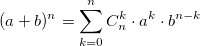также использует биномиальные коэффициенты. Для их расчета можно использовать формулу, выражающую биномиальный коэффициент через факториалы: 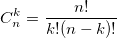или использовать рекуррентную формулу: Из бинома Ньютона и рекуррентной формулы ясно, что биномиальные коэффициенты — целые числа. На данном примере хотелось показать, что даже при решении несложной задачи можно наступить на грабли.
Прежде чем перейти к написанию процедур расчета, рассмотрим так называемый треугольник Паскаля.

          1
       1     1
    1     2     1
  1    3     3     1
1   4     6     4     1

или он же, но немного в другом виде. В левой колонке строки значение n, дальше в строке значения для k=0..n

 n          биномиальные коэффициенты
 0      1
 1      1      1
 2      1      2      1
 3      1      3      3      1
 4      1      4      6      4      1
 5      1      5     10     10      5      1
 6      1      6     15     20     15      6      1
 7      1      7     21     35     35     21      7      1
 8      1      8     28     56     70     56     28      8      1
 9      1      9     36     84    126    126     84     36      9      1
10      1     10     45    120    210    252    210    120     45     10      1
11      1     11     55    165    330    462    462    330    165     55     11      1
12      1     12     66    220    495    792    924    792    495    220     66     12      1
13      1     13     78    286    715   1287   1716   1716   1287    715    286     78     13      1
14      1     14     91    364   1001   2002   3003   3432   3003   2002   1001    364     91     14      1
15      1     15    105    455   1365   3003   5005   6435   6435   5005   3003   1365    455    105     15      1
16      1     16    120    560   1820   4368   8008  11440  12870  11440   8008   4368   1820    560    120     16      1

В полном соответствии с рекуррентной формулой значения равны 1 и любое число равно сумме числа, стоящего над ним и числа «над ним+шаг влево». Например, в 7й строке число 21, а в 6й строке числа 15 и 6: 21=15+6. Видно также, что значения в строке симметричны относительно середины строки, т.е. . Это свойство симметричности бинома Ньютона относительно a и b и оно видно в факториальной формуле.
Ниже для биномиальных коэффициентов я буду также использовать представление C(n,k) (его проще набирать, да и формулу-картинку не везде можно вставить.

Расчет биномиальных коэффициентов через факториальную формулу

поскольку биномиальные коэффициенты неотрицательные, будем использовать в расчетах беззнаковый тип.

// расчет факториала n
unsigned fakt(int n)
{
   unsigned r;
   for (r=1;n>0;--n)  
         r*=n;
   return r;
}
// расчет C(n,k)
unsinged bci(int n,int k)
{
   return fakt(n)/(fakt(k)*fakt(n-k));
}

Вызовем функцию bci(10,4) — она вернет 210 и это правильное значение коэффициента C(10,4). Значит, задача расчета решена? Да, решена. Но не совсем. Мы не ответили на вопрос: при каких максимальных значениях n,k функция bci будет работать правильно? Прежде чем начать искать ответ, условимся, что используемый нами тип unsigned int 4-х байтный и максимальное значение равно 2³²-1=4’294’967’295. При каких n,k C(n,k) превысит его? Обратимся к треугольнику Паскаля. Видно, что максимальные значения достигаются в середине строки, т.е. при k=n/2. Если n четно, то имеется одно максимальное значение, а если n нечетно, то их два. Точное значение C(34,17) равно 2333606220, а точное значение C(35,17) равно 4537567650, т.е. уже больше максимального unsigned int.
Напишем тестовую процедуру

void test()
{
    for (n=10;n<=35;++n) 
    printf("%u %u",n,bci(n,n/2);
 // для C++ можно использовать cout<<n<<" "<<bci(n,n/2)<<endl;
}

Запустим ее и увидим

Значение в очередной строке должно быть примерно в 2 раза больше, чем в предыдущей. Поэтому последний правильно вычисленный коэффициент (см треугольник выше) — это C(12,6) Хотя unsigned int вмещает 4млрд, правильно вычисляются значения меньше 1000. Вот те раз, почему так? Все дело в нашей процедуре bci, точнее в строке, которая сначала вычисляет большое число в числителе, а потом делит его на большое число в знаменателе. Для вычисления C(13,6) сначала вычисляется 13!, а это число > 6млрд и оно не влезает в unsigned int.
Как оптимизировать расчет ? Очень просто: раскроем 13! и сократим числитель и знаменатель на 7! В результате получится . Запрограммируем расчет по этой формуле

unsigned bci(int n,int k) 
{
	if (k>n/2) k=n-k; // возьмем минимальное из k, n-k.. В силу симметричность C(n,k)=C(n,n-k)
	if (k==1)  return n;
	if (k==0)  return 1;
	unsigned r=1;
	for (int i=1; i<=k;++i) {
		r*=n-k+i;
		r/=i;
	}
	return r;
}

и снова протестируем

10 252
11 462
12 924
13 1716
14 3432
15 6435
16 12870
17 24310
18 48620
19 92378
20 184756
21 352716
22 705432
23 1352078
24 2704156
25 5200300
26 10400600
27 20058300
28 40116600
29 77558760
30 155117520
31 14209041
32 28418082
33 39374192
34 78748384
35 79433695

Явно лучше, ошибка возникла при расчете C(31,15). Причина понятна — все то же переполнение. Сначала умножаем на 31 (оп-па — переполнение, потом делим на 15). А что, если использовать рекурсивную формулу? Там только сложение, переполнения быть не должно.
Что ж, пробуем:

unsigned bcr(int n,int k) 
{
	if (k>n/2) k=n-k;
	if (k==1)  return n;
	if (k==0)  return 1;
	return bcr(n-1,k)+bcr(n-1,k-1);
}
void test()
{
    for (n=10;n<=35;++n) 
    printf("%u %u",n,bcr(n,n/2);
 // для C++ можно использовать cout<<n<<" "<<bcr(n,n/2)<<endl;
}

Результат теста

10 252
11 462
12 924
13 1716
14 3432
15 6435
16 12870
17 24310
18 48620
19 92378
20 184756
21 352716
22 705432
23 1352078
24 2704156
25 5200300
26 10400600
27 20058300
28 40116600
29 77558760
30 155117520
31 300540195
32 601080390
33 1166803110
34 2333606220
35 242600354

Все, что влезло в unsigned int, посчиталось правильно. Вот только строчка с n=34 считалась около минуты. При расчете C(n,n/2) делается два рекурсивных вызова, поэтому время расчета экспоненциально зависит от n. Что же делать — получается либо неточно, либо медленно. Выход — в использовании 64 битных переменных.

Замечание по результатам обсуждений: в конце статьи добавлен раздел, где приведен простой и быстрый вариант «bcr с запоминанием» одного из участников обсуждения.

Использование 64 битных типов для расчета C(n,k)

Заменим в функции bci unsigned int на unsigned long long и протестируем в диапазоне n=34..68. n=34 — это максимальное значение, которое правильно считается bci, а C(68,34) ~2.8*10¹⁹ уже не влезает в unsigned long long ~1.84*10¹⁹

unsigned long long bcl(int n,int k) 
{
	if (k>n/2) k=n-k;
	if (k==1)  return n;
	if (k==0)  return 1;
	unsigned long long r=1;
	for (int i=1; i<=k;++i) {
		r*=n-k+i;
		r/=i;
	}
	return r;
}

void test()
{
    for (n=34;n<=68;++n) 
    printf("%llu %llu",n,bcl(n,n/2));
 // для C++ можно использовать cout<<n<<" "<<bcl(n,n/2)<<endl;
}

Результат теста

34 2333606220
35 4537567650
36 9075135300
37 17672631900
38 35345263800
39 68923264410
40 137846528820
41 269128937220
42 538257874440
43 1052049481860
44 2104098963720
45 4116715363800
46 8233430727600
47 16123801841550
48 32247603683100
49 63205303218876
50 126410606437752
51 247959266474052
52 495918532948104
53 973469712824056
54 1946939425648112
55 3824345300380220
56 7648690600760440
57 15033633249770520
58 30067266499541040
59 59132290782430712
60 118264581564861424
61 232714176627630544
62 465428353255261088
63 321255810029051666
64 66050867754679844
65 454676336121653775
66 350360427585442349
67 23341572944240599
68 46683145888481198

Видим, что ошибка возникает при n=63 по той же причине, что и в bci. Сначала умножение на 63 (и переполнение), затем деление на 31.

Дальнейшее повышение точности и расчет при n>67

Ошибка возникла при n=63, а при n=68 результат уже не влезает в unsigned64. Поэтому можно сказать «до n<=62 функция bcl считает правильно, дальнейшее увеличение точности требует либо int128 либо длинной арифметики». А если очень высокая точность не нужна, но хочется считать биномиальные коэффициенты при n=100…1000? Снова берем процедуру bci и меняем в ней типы unsigned int на double:

double bcd(int n,int k) 
{
	if (k>n/2) k=n-k; // возьмем минимальное из k, n-k.. В силу симметричности C(n,k)=C(n,n-k)
	if (k==1)  return n;
	if (k==0)  return 1;
	double r=1;
	for (int i=1; i<=k;++i) {
		r*=n-k+i;
		r/=i;
	}
	return ceil(r-0.2); // округлим до ближайшего целого, отбросив дробную часть
                       // комментарий изменен после обсуждений: такой способ использован,  чтобы расхождение с точным значением 
                       // было как можно позже. Где-то оно превышало 0.5 и простой round не годился 
}
void testd()
{
    for (n=50;n<=1000;n+=50) 
    printf("%d %.16en",n,bcd(n,n/2));
 // для C++ можно использовать cout<<n<<" "<<bcd(n,n/2)<<endl;
}

Результат теста

50 1.2641060643775200e+014
100 1.0089134454556417e+029
150 9.2826069736708704e+043
200 9.0548514656103225e+058
250 9.1208366928185793e+073
300 9.3759702772827310e+088
350 9.7744946171567713e+103
400 1.0295250013541435e+119
450 1.0929255500575370e+134
500 1.1674431578827770e+149
550 1.2533112137626624e+164
600 1.3510794199619429e+179
650 1.4615494992533863e+194
700 1.5857433585316801e+209
750 1.7248900341772600e+224
800 1.8804244186835327e+239
850 2.0539940413411323e+254
900 2.2474718820660189e+269
950 2.4629741379276902e+284
1000 2.7028824094543663e+299

Даже для n=1000 удалось посчитать! Переполнение double произойдет при n=1030.
Расхождение расчета bcd с точным значением начинается с n=57. Он небольшое — всего 8. При n=67 отклонение 896.

Для экстремалов и «олимпийцев»

В принципе, для практических задач точности функции bcd достаточно, но в олимпиадных задачах часто даются тесты «на грани». Т.е. теоретически может встретится задача, где точности double недостаточно и C(n,k) влезает в unsigned long long еле-еле. Как избежать переполнения для таких крайних случаев? Можно использовать рекурсивный алгоритм. Но если он для n=34 считал минуту, то для n=67 будет считать лет 100. Можно запоминать рассчтанные значения (см Дополнение после публиукации).Также можно использовать рекурсию не для всех n и k, а только для «достаточно больших». Вот процедура расчета, которая считает правильно для n<=67. Иногда и для n>67 при малых k (к примеру, считает C(82,21)=1.83*10¹⁹).

unsigned long long bcl(int n,int k) 
{
	if (k>n/2) k=n-k;
	if (k==1)  return n;
	if (k==0)  return 1;
	unsigned long long r;
	if (n+k>=90) {
		// разрядности может не хватить, используем рекурсию
		r=bcl(n-1,k);
		r+=+bcl(n-1,k-1);
	}
	else {
		r=1;
		for (int i=1; i<=k;++i) {
			r*=n-k+i;
			r/=i;
		}
	}
	return r;
}

В какой-то из олимпиадных задач мне потребовалось вычислять много C(n,k) для n >70, т.е. они заведомо не влезали в unsigned long long. Естественно, пришлось использовать «длинную арифметику» (свою). Для этой задачи я написал «рекурсию с памятью»: вычисленные коэффициенты запоминались в массиве и экспоненциального роста времени расчета не было.

Дополнение после публикации

При обсуждении часто упоминаются варианты с запоминанием рассчитанных значений. У меня есть код с динамическим выделением памяти, но я его не привел. На даный момент вот самый простой и эффективный из комментария chersanya: http://habrahabr.ru/post/274689/#comment_8730359http://habrahabr.ru/post/274689/#comment_8730359


unsigned bcr_cache[N_MAX][K_MAX] = {0};

unsigned bcr(int n,int k) 
{
	if (k>n/2) k=n-k;
	if (k==1)  return n;
	if (k==0)  return 1;
        if (bcr_cache[n][k] == 0)
            bcr_cache[n][k] = bcr(n-1,k)+bcr(n-1,k-1);
        return bcr_cache[n][k];
}

Если в программе надо использовать [почти] все коэффициенты треугольника Паскаля (до какого-то уровня), то приведенный рекурсивный алгоритм с запоминанием — самый быстрый способ. Аналогичный код годится и для unsigned long long и даже для длинной арифметики (хотя там, наверное, лучше динамически вычислять и выделять требуемый объем памяти). Конкретные значения N_MAX могут быть такими:
35 — посчитает все коэффициенты C(n,k), n< 35 для unsigned int (32 бита)
68 — посчитает все коэффициенты C(n,k), n< 68 для unsigned long long (64 бита)
200 — посчитает коэффициенты C(n,k), n< 200 и некоторых k для unsigned long long (64 бита). Например, для С(82,21)=~1.83*10¹⁹
K_MAX — это может быть N_MAX/2+1, но не больше 35, поскольку C(68,34) за границей unsigned long long.
Для простоты можно всегда брать K_MAX=35 и не думать «войдет — не войдет» (до тех пор, пока не перейдем к числами с разрядностью >64 бита).

Расчет биномиальных коэффициентов на Python

Это дополнение появилось спустя примерно погода после публикации статьи. Автор начал осваивать Python и для тренироки я решаю олимпиадные задачи, сделанные ранее на C++. Для задач связанных в точными/длинными вычислениями приходится либо всячески исхитряться (как при расчетах биномиальных коэфиициентов), дабы избежать раннего переполнения, либо смиряться с потерей точности (перейдя к типу double) либо писать(или искать) длинную арифметику. В Python длинная арифметика уже есть, поэтому тут для вычисления биномиальных коэффициентов достаточно реализовать запоминание. Запоминать их будем в списке (передается в функцию как папаметр).

# при вызове функции заполняем все, что выше/левее
# в списке биномиальных коэффициентов bcs храним значения, начиная с n=4 и k=2
def Binc(bcs,n,k):
    if (k>n):   return 0
    if k>n//2:  k=n-k # страшую часть строки не храним - она симметрична
    if k==0:    return 1
    if k==1:    return n
    while len(bcs)<n-3:
        # заполняем выше
        for i in range(len(bcs),n-3):
            r=[]
            for j in range(2,i//2+3):
                r.append(Binc(bcs,i+3,j-1)+Binc(bcs,i+3,j))
            bcs.append(r)
    r=bcs[n-4]
    if len(r)<k-1:
        # заполняем левее
        for i in range(len(r),k-1):
            r.append(Binc(bcs,n-1,k-1)+Binc(bcs,n-1,k))
    return bcs[n-4][k-2]
# конец функции

# для контоля рассчитаем C(1000,500)
bcs=[] # пустой список биномиальных коэффициентов
t1=time.clock() 
print(Binc(bcs,1000,500))
t2=time.clock() 
print(t2-t1)

# а это вывод таблички из начала статьи
for n in range(0,16):
    print("n=%2d " % n,end="")
    for k in range(0,n+1):
        print("%5d" % Binc(bcs,n,k),end="")
    print()

Вот вывод (без таблички)
270288240945436569515614693625975275496152008446548287007392875106625428705522193898612483924502370165362606085021546104802209750050679917549894219699518475423665484263751733356162464079737887344364574161119497604571044985756287880514600994219426752366915856603136862602484428109296905863799821216320
0.4200884663301988
Меньше полсекуды для такого коэффициента
C(68,34) (напомню — он не влезает в long long) считается за 0.017 сек и равен 28453041475240576740

Источник

Биномиальными коэффициентами
являются величины

которые выражают число сочетаний
из nэлементов поk.
Эти величины обладают следующими
свойствами.

Свойство
симметрии.

В формуле бинома
это означает, что коэффициенты, стоящие
на одинаковых местах от левого и правого
концов формулы, равны, например:

Действительно,
–
это количество подмножеств, содержащихkэлементов, множества, содержащегоnэлементов. А–
количество дополнительных к ним
подмножеств. Сколько подмножеств,
столько и дополнений.

Свойство
Паскаля.

Пусть
.
Число–
это количество подмножеств из k
элементов множестваX.
Разделим все подмножества на два класса:

1) подмножества,
не содержащие элемент
,
– их будет;

2) подмножества,
содержащие элемент
,
– их будет.

Т.к. эти классы
не пересекаются, то по правилу суммы
количество всех k-элементных
подмножеств множестваXбудет равно

На этом свойстве
основано построение треугольника
Паскаля (рис. 2.2), в n-ой
строке которого стоят коэффициенты
разложения бинома.

Свойство
суммы.

Подставим в
формулу бинома Ньютона

значения
.
Получим

Заметим, что с
точки зрения теории множеств сумма
выражает количество всех подмножествn-элементного
множества. По теореме о мощности булеана
(см. 1.4.4) это количество равно.

Свойство
разности.

Положим в формуле
бинома Ньютона
.
Получим в левой части,
а в правой – биномиальные коэффициенты
с чередующимися знаками, что и доказывает
свойство.

Последнее
свойство удобнее записать, перенеся
все коэффициенты с отрицательными
знаками в левую часть формулы:

тогда свойство легко запоминается
в словесной формулировке: “ сумма
биномиальных коэффициентов с нечетными
номерами равна сумме биномиальных
коэффициентов с четными номерами”.

Задача.
Найти член разложения биномане содержащийx,
если сумма биномиальных коэффициентов
с нечетными номерами равна 512.

Решение. По
свойству разности сумма биномиальных
коэффициентов с четными номерами также
равна 512, значит, сумма всех коэффициентов
равна 512+512=1024. Но по свойству суммы это
число равно.
Поэтому.
Запишем общий член разложения бинома
и преобразуем его:

при
получим:

Член разложения
не содержитx,
если
,
т.е..
Итак, девятый член разложения не содержит xи равен

Свойство
максимума. Если степень биномаn– четное число, то среди биномиальных
коэффициентов есть один максимальный
при.
Если степень бинома нечетное число, то
максимальное значение достигается для
двух биномиальных коэффициентов прии