![]()
Загрузить PDF
![]()
Загрузить PDF
Линейная интерполяция (или просто интерполяция)[1]
— процесс нахождения промежуточных значений величины по ее известным значениям. Многие люди могут провести интерполяцию, полагаясь исключительно на интуицию, но в этой статье описан формализованный математический подход к проведению интерполяции.
Шаги
-

1
Определите величину, для которой вы хотите найти соответствующее значение. Интерполяция может быть проведена для вычисления логарифмов или тригонометрических функций или для вычисления соответствующего объема или давления газа при данной температуре.[2]
Научные калькуляторы в значительной степени заменили логарифмические и тригонометрические таблицы; поэтому в качестве примера проведения интерполяции мы вычислим давление газа при температуре, значение которой не указано в справочных таблицах (или на графиках).- В уравнении, которое мы выведем, «x» будет обозначать известную величину, а «у» — неизвестную величину (интерполированное значение). При построении графика эти значения откладываются соответственно их обозначениям — величина «x» — по оси X, величина «у» — по оси Y.
- В нашем примере под «x» будет подразумеваться температура газа, равная 37 °С.
-
2
В таблице или на графике найдите ближайшие значения, расположенные ниже и выше значения «x». В нашей справочной таблице не приведено давление газа при 37 °С, но приведены значения давления при 30 °С и при 40 °С. Давление газа при температуре 30 °С = 3 кПа, а давление газа при 40 °С = 5 кПа.
- Так как мы обозначили температуру в 37 °С как «x», то теперь обозначим температуру в 30 °С как x1, а температуру в 40 °С как x2.
- Так как мы обозначили неизвестное (интерполированное) давление газа как «у», то теперь обозначим давление в 3 кПа (при 30 °С) как у1, а давление в 5 кПа (при 40 °С) как у2.
- Так как мы обозначили температуру в 37 °С как «x», то теперь обозначим температуру в 30 °С как x1, а температуру в 40 °С как x2.
-
3
Найдем интерполированное значение. Уравнение для нахождения интерполированного значения можно записать в виде y = y1 + ((x – x1)/(x2 – x1) * (y2 – y1))[3]
- Подставим значения x, x1, x2 и получим: (37 – 30)/(40 – 30) = 7/10 = 0,7.
- Подставим значения у1, у2 и получим: (5 – 3) = 2.
- Умножив 0,7 на 2, получим 1,4. Сложим 1,4 и у1: 1,4 + 3 = 4,4 кПа. Проверим ответ: найденное значение 4,4 кПа лежит между 3 кПа (при 30 °С) и 5 кПа (при 40 °С), а так как 37 °С ближе к 40 °С, чем к 30 °С, то и окончательный результат (4,4 кПа) должен быть ближе к 5 кПа, чем к 3 кПа.
Реклама
- Подставим значения x, x1, x2 и получим: (37 – 30)/(40 – 30) = 7/10 = 0,7.


Советы
- Если вы умеете работать с графиками, вы можете сделать грубую интерполяцию, отложив известное значение по оси X и найдя соответствующее значение на оси Y.[4]
В приведенном выше примере можно построить график, на котором по оси X откладывается температура (в десятках градусов), а по оси Y — давление (в единицах кПа). На этом графике вы можете нанести точку 37 градусов, а затем найти точку на оси Y, соответствующую этой точке (она будет лежать между точками 4 и 5 кПа). Приведенное выше уравнение просто формализует процесс мышления и обеспечивает получение точного значения. - В отличие от интерполяции, экстраполяция позволяет вычислить приблизительные значения величины вне диапазона значений, приведенных в таблицах или отображенных на графиках.[5]
Реклама
Об этой статье
Эту страницу просматривали 98 219 раз.
Была ли эта статья полезной?
Текущая версия страницы пока не проверялась опытными участниками и может значительно отличаться от версии, проверенной 9 июля 2022 года; проверки требует 1 правка.
У этого термина существуют и другие значения, см. Интерполяция.
- О функции, см.: Интерполянт.
Интерполя́ция, интерполи́рование (от лат. inter–polis — «разглаженный, подновлённый, обновлённый; преобразованный») — в вычислительной математике нахождение неизвестных промежуточных значений некоторой функции, по имеющемуся дискретному набору её известных значений, определенным способом. Термин «интерполяция» впервые употребил Джон Валлис в своём трактате «Арифметика бесконечных» (1656).
В функциональном анализе интерполяция линейных операторов представляет собой раздел, рассматривающий банаховы пространства как элементы некоторой категории[1].
Многим из тех, кто сталкивается с научными и инженерными расчётами, часто приходится оперировать наборами значений, полученных опытным путём или методом случайной выборки. Как правило, на основании этих наборов требуется построить функцию, на которую могли бы с высокой точностью попадать другие получаемые значения. Такая задача называется аппроксимацией. Интерполяцией называют такую разновидность аппроксимации, при которой кривая построенной функции проходит точно через имеющиеся точки данных.
Существует также близкая к интерполяции задача, которая заключается в аппроксимации какой-либо сложной функции другой, более простой функцией. Если некоторая функция слишком сложна для производительных вычислений, можно попытаться вычислить её значение в нескольких точках, а по ним построить, то есть интерполировать, более простую функцию. Разумеется, использование упрощенной функции не позволяет получить такие же точные результаты, какие давала бы первоначальная функция. Но в некоторых классах задач достигнутый выигрыш в простоте и скорости вычислений может перевесить получаемую погрешность в результатах.
Следует также упомянуть и совершенно другую разновидность математической интерполяции, известную под названием «интерполяция операторов». К классическим работам по интерполяции операторов относятся теорема Рисса — Торина и теорема Марцинкевича[en], являющиеся основой для множества других работ.
Определения[править | править код]
Рассмотрим систему несовпадающих точек  (
( ) из некоторой области
  . Пусть значения функции
  известны только в этих точках:

Задача интерполяции состоит в поиске такой функции  из заданного класса функций, что

</math>A(x)
Пример[править | править код]
1. Пусть мы имеем табличную функцию, наподобие описанной ниже, которая для нескольких значений  определяет соответствующие значения :
|
|

|
|---|---|
| 0 | 0 |
| 1 | 0,8415 |
| 2 | 0,9093 |
| 3 | 0,1411 |
| 4 | −0,7568 |
| 5 | −0,9589 |
| 6 | −0,2794 |
Интерполяция помогает нам узнать, какое значение может иметь такая функция в точке, отличной от указанных точек (например, при x = 2,5).
К настоящему времени существует множество различных способов интерполяции. Выбор наиболее подходящего алгоритма зависит от ответов на вопросы: как точен выбираемый метод, каковы затраты на его использование, насколько гладкой является интерполяционная функция, какого количества точек данных она требует и т. п.
2. Найти промежуточное значение (способом линейной интерполяции).
| 6000 | 15.5 |
| 6378 | ? |
| 8000 | 19.2 |

Способы интерполяции[править | править код]
Интерполяция методом ближайшего соседа[править | править код]
Простейшим способом интерполяции является интерполяция методом ближайшего соседа.
Интерполяция многочленами[править | править код]
На практике чаще всего применяют интерполяцию многочленами. Это связано прежде всего с тем, что многочлены легко вычислять, легко аналитически находить их производные и множество многочленов плотно в пространстве непрерывных функций (теорема Вейерштрасса).
- Линейная интерполяция
- Интерполяционная формула Ньютона
- Метод конечных разностей
- ИМН-1 и ИМН-2
- Многочлен Лагранжа (интерполяционный многочлен)
- Схема Эйткена
- Сплайн-функция
- Кубический сплайн
Обратное интерполирование (вычисление x при заданной y)[править | править код]
- Полином Лагранжа
- Обратное интерполирование по формуле Ньютона
- Обратное интерполирование по формуле Гаусса
Интерполяция функции нескольких переменных[править | править код]
- Билинейная интерполяция
- Бикубическая интерполяция
Другие способы интерполяции[править | править код]
- Рациональная интерполяция
- Тригонометрическая интерполяция
Смежные концепции[править | править код]
- Экстраполяция — методы нахождения точек за пределами заданного интервала (продление кривой)
- Ретрополяция — методы нахождения по известным значениям переменной её неизвестных значений в начале динамического ряда.
- Аппроксимация — методы построения приближённых кривых
См. также[править | править код]
- Интерполяционные формулы
- Регрессия (математика)
- Метод наименьших квадратов
- Сглаживание данных эксперимента
Примечания[править | править код]
- ↑ Берг, 1980, с. 6—7.
Литература[править | править код]
- Й. Берг, Й. Лёфстрём. Интерполяционные пространства. Введение. — М.: Мир, 1980. — 264 с.
- Ибрагимов И. И. Методы интерполяций функций и некоторые их применения. — М.: Высшая школа, 1971. — 520 c.
- Уолш Дж. Л.[en] Интерполяция и аппроксимация рациональными функциями в комплексной области. — М.: Иностранная литература, 1961. — 508 c.
- Трибель Х. Теория интерполяции, функциональные пространства, дифференциальные операторы. — М.: Мир, 1980. — 664 c.
Как найти число методом интерполяции???
Ученик
(240),
закрыт
8 лет назад
Дополнен 12 лет назад
допустим дано
7 – 2400
8,87 – ?
10 – 2600
как найти ???
Дополнен 12 лет назад
Желательно какая нибудь формула, по которой можно будет найти подобные выражения
Дополнен 12 лет назад
Ответ я знаю, мне нужна формула как вы его получили. Благодарю за ранее
Велон
Просветленный
(36271)
12 лет назад
число 2524,67 – ответ
как делается – на разницу 10-7 = 3 приходится 2600-2400 = 200
на одну единицу – 200/3 = 66,67
8.87 – 7 =1,87 Х 66,67 = 124,67
2400 +124,67 = 2524,67
Jurijus Zaksas
Искусственный Интеллект
(393285)
12 лет назад
Зависит от того, что за интерполяция.
В общем случае на основе неких известных точек строится некая стандартная непрерывная функция и из этой функции вычисляется нужная промежуточная точка.
Если известны только 2 точки, используется линейная интерполяция.
Уравнение прямой y=kx+b
Коеэфф. k=dy/dx
b вычисляется подстановкой в уравнение k и любой из известных точек.
Когда коэфф. посчитаны и уравнение известно, остается только подставить в него известную координату искомой точки.

Интерполяция – способ определения промежуточных значений по дискретному (Дискретность – разделённый, прерывистый) набору данных.
Линейная интерполяция – самый простой и наиболее часто используемый ее тип.
Уравнение линейной интерполяции имеет вид:
y = y1 + ((x – x1)/(x2 – x1) * (y2 – y1)),
где
y – искомое;
x – показатель для которого определяется значение (искомое);
x1 – наименьший показатель;
x2 – наибольший показатель;
y1 – значение наименьшего показателя;
y2 – значение наибольшего показателя.
Пример определения промежуточного значения,
методом линейной интерполяции
Необходимо найти коэффициент перехода – C от веса снегового покрова на горизонтальной поверхности земли, к нормативной нагрузке на покрытие, для угла наклона кровли – 35°. Известно, что для угла наклона кровли 30° коэффициент C = 1, а для угла наклона кровли 60° коэффициент C = 0.
Получаем значения для формулы:
y = ? (искомое, коэффициент С для угла наклона кровли – 35°);
x = 35 (угол наклона кровли – 35°, для которого находим коэффициент С);
x1 = 30 (наименьший угол наклона кровли – 30°);
x2 = 60 (наибольший угол наклона кровли – 60°).
y1 = 1 (коэффициент С для наименьшего угла наклона кровли – 30°);
y2 = 0 (коэффициент С для наибольшего угла наклона кровли – 60°);
Подставляем в формулу значения:
1 + ((35 – 30) / (60 – 30) х (0 – 1)) = 0,8333
Получаем коэффициент С = 0,83.
From Wikipedia, the free encyclopedia
In the mathematical field of numerical analysis, interpolation is a type of estimation, a method of constructing (finding) new data points based on the range of a discrete set of known data points.[1][2]
In engineering and science, one often has a number of data points, obtained by sampling or experimentation, which represent the values of a function for a limited number of values of the independent variable. It is often required to interpolate; that is, estimate the value of that function for an intermediate value of the independent variable.
A closely related problem is the approximation of a complicated function by a simple function. Suppose the formula for some given function is known, but too complicated to evaluate efficiently. A few data points from the original function can be interpolated to produce a simpler function which is still fairly close to the original. The resulting gain in simplicity may outweigh the loss from interpolation error and give better performance in calculation process.
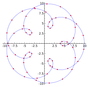
An interpolation of a finite set of points on an epitrochoid. The points in red are connected by blue interpolated spline curves deduced only from the red points. The interpolated curves have polynomial formulas much simpler than that of the original epitrochoid curve.
Example[edit]
This table gives some values of an unknown function .
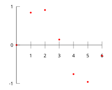
Plot of the data points as given in the table
|
|
|
||||
|---|---|---|---|---|---|
| 0 | 0 | ||||
| 1 | 0 | . | 8415 | ||
| 2 | 0 | . | 9093 | ||
| 3 | 0 | . | 1411 | ||
| 4 | −0 | . | 7568 | ||
| 5 | −0 | . | 9589 | ||
| 6 | −0 | . | 2794 |
Interpolation provides a means of estimating the function at intermediate points, such as 
We describe some methods of interpolation, differing in such properties as: accuracy, cost, number of data points needed, and smoothness of the resulting interpolant function.
Piecewise constant interpolation[edit]

The simplest interpolation method is to locate the nearest data value, and assign the same value. In simple problems, this method is unlikely to be used, as linear interpolation (see below) is almost as easy, but in higher-dimensional multivariate interpolation, this could be a favourable choice for its speed and simplicity.
Linear interpolation[edit]

Plot of the data with linear interpolation superimposed
One of the simplest methods is linear interpolation (sometimes known as lerp). Consider the above example of estimating f(2.5). Since 2.5 is midway between 2 and 3, it is reasonable to take f(2.5) midway between f(2) = 0.9093 and f(3) = 0.1411, which yields 0.5252.
Generally, linear interpolation takes two data points, say (xa,ya) and (xb,yb), and the interpolant is given by:


This previous equation states that the slope of the new line between  and
and  is the same as the slope of the line between and
Linear interpolation is quick and easy, but it is not very precise. Another disadvantage is that the interpolant is not differentiable at the point xk.
The following error estimate shows that linear interpolation is not very precise. Denote the function which we want to interpolate by g, and suppose that x lies between xa and xb and that g is twice continuously differentiable. Then the linear interpolation error is
![|f(x)-g(x)|leq C(x_{b}-x_{a})^{2}quad {text{where}}quad C={frac {1}{8}}max _{rin [x_{a},x_{b}]}|g''(r)|.](https://wikimedia.org/api/rest_v1/media/math/render/svg/15e835bf7d5d64ca8fef6bd55cfd937460b4752e)
In words, the error is proportional to the square of the distance between the data points. The error in some other methods, including polynomial interpolation and spline interpolation (described below), is proportional to higher powers of the distance between the data points. These methods also produce smoother interpolants.
Polynomial interpolation[edit]

Plot of the data with polynomial interpolation applied
Polynomial interpolation is a generalization of linear interpolation. Note that the linear interpolant is a linear function. We now replace this interpolant with a polynomial of higher degree.
Consider again the problem given above. The following sixth degree polynomial goes through all the seven points:

Substituting x = 2.5, we find that f(2.5) = ~0.59678.
Generally, if we have n data points, there is exactly one polynomial of degree at most n−1 going through all the data points. The interpolation error is proportional to the distance between the data points to the power n. Furthermore, the interpolant is a polynomial and thus infinitely differentiable. So, we see that polynomial interpolation overcomes most of the problems of linear interpolation.
However, polynomial interpolation also has some disadvantages. Calculating the interpolating polynomial is computationally expensive (see computational complexity) compared to linear interpolation. Furthermore, polynomial interpolation may exhibit oscillatory artifacts, especially at the end points (see Runge’s phenomenon).
Polynomial interpolation can estimate local maxima and minima that are outside the range of the samples, unlike linear interpolation. For example, the interpolant above has a local maximum at x ≈ 1.566, f(x) ≈ 1.003 and a local minimum at x ≈ 4.708, f(x) ≈ −1.003. However, these maxima and minima may exceed the theoretical range of the function; for example, a function that is always positive may have an interpolant with negative values, and whose inverse therefore contains false vertical asymptotes.
More generally, the shape of the resulting curve, especially for very high or low values of the independent variable, may be contrary to commonsense; that is, to what is known about the experimental system which has generated the data points. These disadvantages can be reduced by using spline interpolation or restricting attention to Chebyshev polynomials.
Spline interpolation[edit]

Plot of the data with spline interpolation applied
Remember that linear interpolation uses a linear function for each of intervals [xk,xk+1]. Spline interpolation uses low-degree polynomials in each of the intervals, and chooses the polynomial pieces such that they fit smoothly together. The resulting function is called a spline.
For instance, the natural cubic spline is piecewise cubic and twice continuously differentiable. Furthermore, its second derivative is zero at the end points. The natural cubic spline interpolating the points in the table above is given by
![f(x)={begin{cases}-0.1522x^{3}+0.9937x,&{text{if }}xin [0,1],\-0.01258x^{3}-0.4189x^{2}+1.4126x-0.1396,&{text{if }}xin [1,2],\0.1403x^{3}-1.3359x^{2}+3.2467x-1.3623,&{text{if }}xin [2,3],\0.1579x^{3}-1.4945x^{2}+3.7225x-1.8381,&{text{if }}xin [3,4],\0.05375x^{3}-0.2450x^{2}-1.2756x+4.8259,&{text{if }}xin [4,5],\-0.1871x^{3}+3.3673x^{2}-19.3370x+34.9282,&{text{if }}xin [5,6].end{cases}}](https://wikimedia.org/api/rest_v1/media/math/render/svg/3cd654c9f03b663dc277263ec988f010e0d934e1)
In this case we get f(2.5) = 0.5972.
Like polynomial interpolation, spline interpolation incurs a smaller error than linear interpolation, while the interpolant is smoother and easier to evaluate than the high-degree polynomials used in polynomial interpolation. However, the global nature of the basis functions leads to ill-conditioning. This is completely mitigated by using splines of compact support, such as are implemented in Boost.Math and discussed in Kress.[3]
Mimetic interpolation[edit]
Depending on the underlying discretisation of fields, different interpolants may be required. In contrast to other interpolation methods, which estimate functions on target points, mimetic interpolation evaluates the integral of fields on target lines, areas or volumes, depending on the type of field (scalar, vector, pseudo-vector or pseudo-scalar).
A key feature of mimetic interpolation is that vector calculus identities are satisfied, including Stokes’ theorem and the divergence theorem. As a result, mimetic interpolation conserves line, area and volume integrals.[4] Conservation of line integrals might be desirable when interpolating the electric field, for instance, since the line integral gives the electric potential difference at the endpoints of the integration path.[5] Mimetic interpolation ensures that the error of estimating the line integral of an electric field is the same as the error obtained by interpolating the potential at the end points of the integration path, regardless of the length of the integration path.
Linear, bilinear and trilinear interpolation are also considered mimetic, even if it is the field values that are conserved (not the integral of the field). Apart from linear interpolation, area weighted interpolation can be considered one of the first mimetic interpolation methods to have been developed.[6]
Function approximation[edit]
Interpolation is a common way to approximate functions. Given a function ![{displaystyle f:[a,b]to mathbb {R} }](https://wikimedia.org/api/rest_v1/media/math/render/svg/b592d102ccd1ba134d401c5b3ea177baaba3ffac) with a set of points
with a set of points ![{displaystyle x_{1},x_{2},dots ,x_{n}in [a,b]}](https://wikimedia.org/api/rest_v1/media/math/render/svg/df22c48c2c827e30fa634d0964908f94af232750) one can form a function
one can form a function ![{displaystyle s:[a,b]to mathbb {R} }](https://wikimedia.org/api/rest_v1/media/math/render/svg/cb454b2565ba3ced5a91e87ee9b2a685a14d03bb) such that
such that  for
for  (that is, that
  interpolates at these points). In general, an interpolant need not be a good approximation, but there are well known and often reasonable conditions where it will. For example, if
 ![{displaystyle fin C^{4}([a,b])}](https://wikimedia.org/api/rest_v1/media/math/render/svg/cf9d66eda475f0e830cf15ecdec3d8fbf5e6ba7e) (four times continuously differentiable) then cubic spline interpolation has an error bound given by
(four times continuously differentiable) then cubic spline interpolation has an error bound given by  where
where  and
and  is a constant.[7]
Via Gaussian processes[edit]
Gaussian process is a powerful non-linear interpolation tool. Many popular interpolation tools are actually equivalent to particular Gaussian processes. Gaussian processes can be used not only for fitting an interpolant that passes exactly through the given data points but also for regression; that is, for fitting a curve through noisy data. In the geostatistics community Gaussian process regression is also known as Kriging.
Other forms[edit]
Other forms of interpolation can be constructed by picking a different class of interpolants. For instance, rational interpolation is interpolation by rational functions using Padé approximant, and trigonometric interpolation is interpolation by trigonometric polynomials using Fourier series. Another possibility is to use wavelets.
The Whittaker–Shannon interpolation formula can be used if the number of data points is infinite or if the function to be interpolated has compact support.
Sometimes, we know not only the value of the function that we want to interpolate, at some points, but also its derivative. This leads to Hermite interpolation problems.
When each data point is itself a function, it can be useful to see the interpolation problem as a partial advection problem between each data point. This idea leads to the displacement interpolation problem used in transportation theory.
In higher dimensions[edit]

Comparison of some 1- and 2-dimensional interpolations.
Black and red/yellow/green/blue dots correspond to the interpolated point and neighbouring samples, respectively.
Their heights above the ground correspond to their values.
Multivariate interpolation is the interpolation of functions of more than one variable.
Methods include bilinear interpolation and bicubic interpolation in two dimensions, and trilinear interpolation in three dimensions.
They can be applied to gridded or scattered data. Mimetic interpolation generalizes to  dimensional spaces where
  .[8][9]
-

Nearest neighbor
-

Bilinear
-

Bicubic


In digital signal processing[edit]
In the domain of digital signal processing, the term interpolation refers to the process of converting a sampled digital signal (such as a sampled audio signal) to that of a higher sampling rate (Upsampling) using various digital filtering techniques (for example, convolution with a frequency-limited impulse signal). In this application there is a specific requirement that the harmonic content of the original signal be preserved without creating aliased harmonic content of the original signal above the original Nyquist limit of the signal (that is, above fs/2 of the original signal sample rate). An early and fairly elementary discussion on this subject can be found in Rabiner and Crochiere’s book Multirate Digital Signal Processing.[10]
[edit]
The term extrapolation is used to find data points outside the range of known data points.
In curve fitting problems, the constraint that the interpolant has to go exactly through the data points is relaxed. It is only required to approach the data points as closely as possible (within some other constraints). This requires parameterizing the potential interpolants and having some way of measuring the error. In the simplest case this leads to least squares approximation.
Approximation theory studies how to find the best approximation to a given function by another function from some predetermined class, and how good this approximation is. This clearly yields a bound on how well the interpolant can approximate the unknown function.
Generalization[edit]
If we consider as a variable in a topological space, and the function mapping to a Banach space, then the problem is treated as “interpolation of operators”.[11] The classical results about interpolation of operators are the Riesz–Thorin theorem and the Marcinkiewicz theorem. There are also many other subsequent results.
See also[edit]
- Barycentric coordinates – for interpolating within on a triangle or tetrahedron
- Brahmagupta’s interpolation formula
- Fractal interpolation
- Imputation (statistics)
- Lagrange interpolation
- Missing data
- Newton–Cotes formulas
- Radial basis function interpolation
- Simple rational approximation
References[edit]
- ^ Sheppard, William Fleetwood (1911). “Interpolation” . In Chisholm, Hugh (ed.). Encyclopædia Britannica. Vol. 14 (11th ed.). Cambridge University Press. pp. 706–710.
- ^ Steffensen, J. F. (2006). Interpolation (Second ed.). Mineola, N.Y. ISBN 978-0-486-15483-1. OCLC 867770894.
- ^ Kress, Rainer (1998). Numerical Analysis. ISBN 9781461205999.
- ^ Pletzer, Alexander; Hayek, Wolfgang (2019-01-01). “Mimetic Interpolation of Vector Fields on Arakawa C/D Grids”. Monthly Weather Review. 147 (1): 3–16. Bibcode:2019MWRv..147….3P. doi:10.1175/MWR-D-18-0146.1. ISSN 1520-0493. S2CID 125214770.
- ^ Stern, Ari; Tong, Yiying; Desbrun, Mathieu; Marsden, Jerrold E. (2015), Chang, Dong Eui; Holm, Darryl D.; Patrick, George; Ratiu, Tudor (eds.), “Geometric Computational Electrodynamics with Variational Integrators and Discrete Differential Forms”, Geometry, Mechanics, and Dynamics, New York, NY: Springer New York, vol. 73, pp. 437–475, doi:10.1007/978-1-4939-2441-7_19, ISBN 978-1-4939-2440-0, S2CID 15194760, retrieved 2022-06-15
- ^ Jones, Philip (1999). “First- and Second-Order Conservative Remapping Schemes for Grids in Spherical Coordinates”. Monthly Weather Review. 127 (9): 2204–2210. Bibcode:1999MWRv..127.2204J. doi:10.1175/1520-0493(1999)127<2204:FASOCR>2.0.CO;2. S2CID 122744293.
- ^ Hall, Charles A.; Meyer, Weston W. (1976). “Optimal Error Bounds for Cubic Spline Interpolation”. Journal of Approximation Theory. 16 (2): 105–122. doi:10.1016/0021-9045(76)90040-X.
- ^ Whitney, Hassler (1957). Geometric Integration Theory. Dover Books on Mathematics. ISBN 978-0486445830.
- ^ Pletzer, Alexander; Fillmore, David (2015). “Conservative interpolation of edge and face data on n dimensional structured grids using differential forms”. Journal of Computational Physics. 302: 21–40. Bibcode:2015JCoPh.302…21P. doi:10.1016/j.jcp.2015.08.029.
- ^ R.E. Crochiere and L.R. Rabiner. (1983). Multirate Digital Signal Processing. Englewood Cliffs, NJ: Prentice–Hall.
- ^ Colin Bennett, Robert C. Sharpley, Interpolation of Operators, Academic Press 1988
External links[edit]
- Online tools for linear, quadratic, cubic spline, and polynomial interpolation with visualisation and JavaScript source code.
- Sol Tutorials – Interpolation Tricks
- Compactly Supported Cubic B-Spline interpolation in Boost.Math[permanent dead link]
- Barycentric rational interpolation in Boost.Math
- Interpolation via the Chebyshev transform in Boost.Math
