Код Хэмминга. Пример работы алгоритма
Время на прочтение
4 мин
Количество просмотров 512K
Вступление.
Прежде всего стоит сказать, что такое Код Хэмминга и для чего он, собственно, нужен. На Википедии даётся следующее определение:
Коды Хэмминга — наиболее известные и, вероятно, первые из самоконтролирующихся и самокорректирующихся кодов. Построены они применительно к двоичной системе счисления.
Другими словами, это алгоритм, который позволяет закодировать какое-либо информационное сообщение определённым образом и после передачи (например по сети) определить появилась ли какая-то ошибка в этом сообщении (к примеру из-за помех) и, при возможности, восстановить это сообщение. Сегодня, я опишу самый простой алгоритм Хемминга, который может исправлять лишь одну ошибку.
Также стоит отметить, что существуют более совершенные модификации данного алгоритма, которые позволяют обнаруживать (и если возможно исправлять) большее количество ошибок.
Сразу стоит сказать, что Код Хэмминга состоит из двух частей. Первая часть кодирует исходное сообщение, вставляя в него в определённых местах контрольные биты (вычисленные особым образом). Вторая часть получает входящее сообщение и заново вычисляет контрольные биты (по тому же алгоритму, что и первая часть). Если все вновь вычисленные контрольные биты совпадают с полученными, то сообщение получено без ошибок. В противном случае, выводится сообщение об ошибке и при возможности ошибка исправляется.
Как это работает.
Для того, чтобы понять работу данного алгоритма, рассмотрим пример.
Подготовка
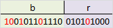
Допустим, у нас есть сообщение «habr», которое необходимо передать без ошибок. Для этого сначала нужно наше сообщение закодировать при помощи Кода Хэмминга. Нам необходимо представить его в бинарном виде.
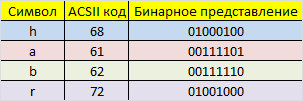
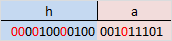
На этом этапе стоит определиться с, так называемой, длиной информационного слова, то есть длиной строки из нулей и единиц, которые мы будем кодировать. Допустим, у нас длина слова будет равна 16. Таким образом, нам необходимо разделить наше исходное сообщение («habr») на блоки по 16 бит, которые мы будем потом кодировать отдельно друг от друга. Так как один символ занимает в памяти 8 бит, то в одно кодируемое слово помещается ровно два ASCII символа. Итак, мы получили две бинарные строки по 16 бит:
 и
и 
После этого процесс кодирования распараллеливается, и две части сообщения («ha» и «br») кодируются независимо друг от друга. Рассмотрим, как это делается на примере первой части.
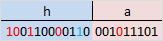
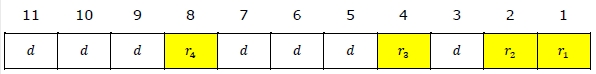
Прежде всего, необходимо вставить контрольные биты. Они вставляются в строго определённых местах — это позиции с номерами, равными степеням двойки. В нашем случае (при длине информационного слова в 16 бит) это будут позиции 1, 2, 4, 8, 16. Соответственно, у нас получилось 5 контрольных бит (выделены красным цветом):
Было:
Стало:
Таким образом, длина всего сообщения увеличилась на 5 бит. До вычисления самих контрольных бит, мы присвоили им значение «0».
Вычисление контрольных бит.
Теперь необходимо вычислить значение каждого контрольного бита. Значение каждого контрольного бита зависит от значений информационных бит (как неожиданно), но не от всех, а только от тех, которые этот контрольных бит контролирует. Для того, чтобы понять, за какие биты отвечает каждых контрольный бит необходимо понять очень простую закономерность: контрольный бит с номером N контролирует все последующие N бит через каждые N бит, начиная с позиции N. Не очень понятно, но по картинке, думаю, станет яснее:
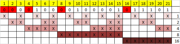
Здесь знаком «X» обозначены те биты, которые контролирует контрольный бит, номер которого справа. То есть, к примеру, бит номер 12 контролируется битами с номерами 4 и 8. Ясно, что чтобы узнать какими битами контролируется бит с номером N надо просто разложить N по степеням двойки.
Но как же вычислить значение каждого контрольного бита? Делается это очень просто: берём каждый контрольный бит и смотрим сколько среди контролируемых им битов единиц, получаем некоторое целое число и, если оно чётное, то ставим ноль, в противном случае ставим единицу. Вот и всё! Можно конечно и наоборот, если число чётное, то ставим единицу, в противном случае, ставим 0. Главное, чтобы в «кодирующей» и «декодирующей» частях алгоритм был одинаков. (Мы будем применять первый вариант).
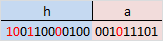
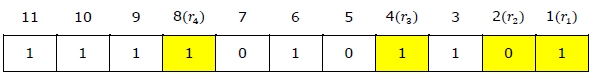
Высчитав контрольные биты для нашего информационного слова получаем следующее:
и для второй части:
Вот и всё! Первая часть алгоритма завершена.
Декодирование и исправление ошибок.
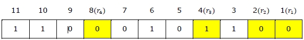
Теперь, допустим, мы получили закодированное первой частью алгоритма сообщение, но оно пришло к нас с ошибкой. К примеру мы получили такое (11-ый бит передался неправильно):
Вся вторая часть алгоритма заключается в том, что необходимо заново вычислить все контрольные биты (так же как и в первой части) и сравнить их с контрольными битами, которые мы получили. Так, посчитав контрольные биты с неправильным 11-ым битом мы получим такую картину:
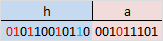
Как мы видим, контрольные биты под номерами: 1, 2, 8 не совпадают с такими же контрольными битами, которые мы получили. Теперь просто сложив номера позиций неправильных контрольных бит (1 + 2 + 8 = 11) мы получаем позицию ошибочного бита. Теперь просто инвертировав его и отбросив контрольные биты, мы получим исходное сообщение в первозданном виде! Абсолютно аналогично поступаем со второй частью сообщения.
Заключение.
В данном примере, я взял длину информационного сообщения именно 16 бит, так как мне кажется, что она наиболее оптимальная для рассмотрения примера (не слишком длинная и не слишком короткая), но конечно же длину можно взять любую. Только стоит учитывать, что в данной простой версии алгоритма на одно информационное слово можно исправить только одну ошибку.
Примечание.
На написание этого топика меня подвигло то, что в поиске я не нашёл на Хабре статей на эту тему (чему я был крайне удивлён). Поэтому я решил отчасти исправить эту ситуацию и максимально подробно показать как этот алгоритм работает. Я намеренно не приводил ни одной формулы, дабы попытаться своими словами донести процесс работы алгоритма на примере.
Источники.
1. Википедия
2. Calculating the Hamming Code
Пример
. Предположим, в канале связи под действием
помех произошло искажение и вместо
0100101 было принято 01001(1)1.
Решение:
Для обнаружения ошибки производят уже
знакомые нам проверки на четность.
Первая
проверка:
сумма П1+П3+П5+П7
= 0+0+1+1 четна.
В младший разряд номера ошибочной
позиции запишем 0.
Вторая
проверка:
сумма П2+П3+П6+П7
= 1+0+1+1 нечетна.
Во второй разряд номера ошибочной
позиции запишем 1
Третья
проверка:
сумма П4+П5+П6+П7
= 0+1+1+1 нечетна.
В третий разряд номера ошибочной позиции
запишем 1. Номер ошибочной позиции 110=
6. Следовательно,
символ шестой позиции следует изменить
на обратный, и получим правильную кодовую
комбинацию.
Код, исправляющий
одиночную и обнаруживающий двойную
ошибки
Если по изложенным
выше правилам строить корректирующий
код с обнаружением и исправлением
одиночной ошибки для равномерного
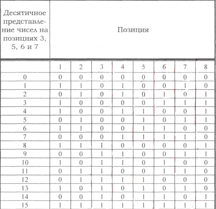
двоичного кода, то первые 16 кодовых
комбинаций будут иметь вид, показанный
в таблице. Такой код может быть использован
для построения кода с исправлением
одиночной ошибки и обнаружением двойной.
Для
этого, кроме указанных выше проверок
по контрольным позициям, следует провести
еще одну проверку на четность для всей
строки в целом. Чтобы осуществить такую
проверку, следует к каждой строке кода
добавить контрольные символы, записанные
в дополнительной колонке (таблица,
колонка 8). Тогда в случае одной ошибки
проверки по позициям укажут номер
ошибочной позиции, а проверка на четность
– на наличие ошибки. Если проверки позиций
укажут на наличие ошибки, а проверка на
четность не фиксирует ее, значит в
кодовой комбинации две ошибки.
Лекция 8
8.1 Двоичные циклические коды
Вышеприведенная
процедура построения линейного кода
матричным методом имеет ряд недостатков.
Она неоднозначна (МДР можно задать
различным образом) и неудобна
в реализации в виде технических устройств.
Этих недостатков лишены
линейные корректирующие коды, принадлежащие
к классу циклических.
Циклическими
называют
линейные (n,k)-коды,
обладающие
следующим свойством:
для любого кодового слова:
![]()
существует другое
кодовое слово:
![]()
полученное
циклическим сдвигом элементов исходного
кодового слова ||КС||
вправо
или влево, которое также принадлежит
этому коду.
Для
описания циклических кодов используют
полиномы с фиктивной переменной
X.
Например,
пусть кодовое слово ||КС||
=
||011010||.
Его
можно описать полиномом
![]()
Таким
образом, разряды кодового слова в
описывающем его полиноме используются
в качестве коэффициентов при степенях
фиктивной переменной
X.
Наибольшая
степень фиктивной переменной X
в
слагаемом с ненулевым
коэффициентом называется степенью
полинома. В вышеприведенном примере
получился полином 4-й степени.
Теперь
действия над кодовыми словами сводятся
к действиям над полиномами.
Вместо алгебры матриц здесь используется
алгебра полиномов.
Рассмотрим
алгебраические действия над полиномами,
используемые в теории
циклических кодов. Суммирование
полиномов разберем на примере
С(Х)=А(Х)+В(Х).
Пусть
||A||
= ||011010||,
||В|| =
||110111|.
Тогда
![]()
![]()
![]()
—————————————————————
![]()
Таким
образом, при суммировании коэффициентов
при X
в одинаковой степени
результат берется по модулю 2. При таком
правиле вычитание эквивалентно
суммированию.
Умножение
выполняется как обычно, но с использованием
суммирования
по модулю 2.
Рассмотрим
умножение на примере умножения полинома
(X3+X1+X0)
на
полином X1+X0
X3
+ 0*X2+X1+X0
*
X1+X0
—————————————————
X3+
0*X2+X1+Х0
X4+0*Х3+
X2+Х1
____________________________________
Х4+
X3+
X2+0*X1+X0
Операция
– обратная умножению -деление. Деление
полиномов выполняется как обычно, за
исключением того, что вычитание
выполняется по модулю 2. Вспомним, что
вычитание по модулю 2 эквивалентно
сложению по модулю 2
Пример
деления полинома X6+X4+X3
на полином
X3+X2+1
X6+0*X5+X4
+ X3+0*X2+0*X1+0
| X3+X2+1
X6+X5+0*X4+X3 результат== |X3+X2
———————————–
X5
+X4
+ 0*X3+0*X2
X5
+X4
+ 0*X3+
X2
—————————————-
остаток==
X2
=
100
Циклический
сдвиг влево на одну позицию коэффициентов
полинома степени n-1
получается
путем его умножения на X
с
последующим вычитанием из
результата полинома Xn+1,
если его порядок >
п.
Проверим это на
примере.
Пусть требуется
выполнить циклический сдвиг влево на
одну позицию
коэффициентов
полинома
C(X)=X5+Х3+X2+1
→ (101101)
В результате должен
получиться полином
C1(X)=X4+Х3+X1+1
→ (011011)
Это легко
доказывается:
C1(X)=C(X)*X-(X6+1)=(X6+Х4+X3+X)+(
X6+1)=X4+Х3+X1+1
В
основе циклического кода лежит образующий
полином r-го
порядка
(напомним, что r–
число дополнительных разрядов). Будем
обозначать
его gr(X).
Образование
кодовых слов (кодирование) КС
выполняется
путем умножения
информационного полинома с коэффициентами,
являющимися информационной
последовательностью
И(Х)
порядка
i<k
на
образующий полином gr(X)
КСr+k(Х)=gr(X)+ИСk(Х).
Принятое кодовое
слово может отличаться от переданного
искаженными разрядами в результате
воздействия помех.
ПКС(Х)=КС(Х)+ВО(Х).
где
ВО(Х)
– полином
вектора ошибки, а суммирование, как
обычно, ведется
по модулю 2.
Декодирование,
как и раньше начинается с нахождения
опознавателя,
в данном случае в виде полинома ОП(Х).
Этот
полином вычисляется как
остаток от деления полинома принятого
кодового слова ПКС(Х)
на
образующий
полином g(Х):
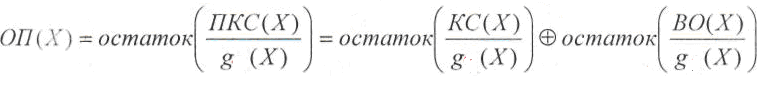
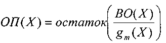
Первое
слагаемое остатка не имеет, т.к. кодовое
слово было образовано путем умножения
полинома информационной последовательности
на
образующий полином. Следовательно, и в
данном случае опознаватель
полностью зависит от вектора ошибки.
Образующий
полином выбирается таким, чтобы при
данном r
как
можно
большее число отношений ВО(Х)/g(Х)
давало
различные остатки.
Такому
требованию отвечают так называемые
неприводимые
полиномы,
которые
не делятся без остатка ни на один полином
степени r
и ниже, а
делятся только сами на себя и на 1.
Приведенная
здесь процедура образования кодового
слова неудобна тем,
что такой код получается несистематическим,
т.е. таким, в кодовых словах
которого нельзя выделить информационные
и дополнительные разряды.
Этот недостаток
был устранен следующим образом.
Способ
кодирования, приводящий к получению
систематического линейного циклического
кода, состоит в приписывании к
информационной
последовательности И
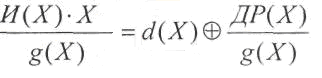
дополнительных разрядов ДР.
Эти
дополнительные разряды предлагается
находить по следующей формуле:
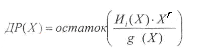
Порядок
полинома ДР(Х)
гарантировано
меньше r
(поскольку
это остаток).
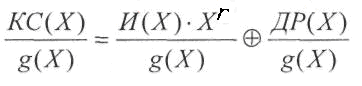
Приписывание
дополнительных разрядов к информационной
последовательности,
используя алгебру полиномов, можно
описать формулой:
![]()
Одним
из свойств циклических линейных кодов
является то, что результат
деления любого разрешенного кодового
слова КС
на
образующий полином также, является
разрешенным кодовым словом.
Покажем,
что получаемые по вышеприведенному
алгоритму кодовые
слова являются кодовыми словами
циклического линейного кода. Для
этого нужно убедиться в том, что
произвольное разрешенное кодовое
слово делится на образующий полином
g(X)
без остатка:
Рассмотрим первое
слагаемое:
где
d(Х)
– целая
часть результата деления.
Подставим полученную
сумму на место первого слагаемого:
![]() Суммирование
Суммирование
последних двух слагаемых дает нулевой
результат (напомним,
что суммирование выполняется по модулю
2).
Значит
![]() –
–
целая часть деления. Остатка нет. Это
означает,
что описанный выше способ кодирования
соответствует циклическому
коду.
Соседние файлы в предмете [НЕСОРТИРОВАННОЕ]
- #
- #
- #
- #
- #
- #
- #
- #
- #
- #
- #
| Двоичный код Хэмминга | |
|---|---|
 Код Хэмминга  с с  |
|
| Назван в честь | Ричард Хэмминг |
| Тип | линейный блочный код |
| Длина блока |
 |
| Длина сообщения |
 |
| Доля |
 |
| Расстояние | 3 |
| Размер алфавита | 2 |
| Обозначение |
![{displaystyle [2^{r}-1,2^{r}-r-1,3]_{2}}](https://wikimedia.org/api/rest_v1/media/math/render/svg/f4b7099796302beb1cea00796f3d9a67b448e08c) |
Код Хэ́мминга — самоконтролирующийся и самокорректирующийся код. Построен применительно к двоичной системе счисления.
Позволяет исправлять одиночную ошибку (ошибка в одном бите слова) и находить двойную[1].
Назван в честь американского математика Хэмминга Ричарда Уэсли, предложившего код.
История[править | править код]
В середине 1940-х годов в лаборатории Белла была создана счётная машина Bell Model V. Это была электромеханическая машина, использующая релейные блоки, скорость которых была очень низка: одна операция за несколько секунд. Данные вводились в машину с помощью перфокарт с ненадёжными устройствами чтения, поэтому в процессе чтения часто происходили ошибки. В рабочие дни использовались специальные коды, чтобы обнаруживать и исправлять найденные ошибки, при этом оператор узнавал об ошибке по свечению лампочек, исправлял и снова запускал машину. В выходные дни, когда не было операторов, при возникновении ошибки машина автоматически выходила из программы и запускала другую.
Хэмминг часто работал в выходные дни и всё больше раздражался, так как должен был перезагружать свою программу из-за ненадёжности считывателя перфокарт. На протяжении нескольких лет он искал эффективный алгоритм исправления ошибок. В 1950 году он опубликовал способ кодирования, который известен как код Хэмминга.
Систематические коды[править | править код]
Систематические коды образуют большую группу из блочных, разделимых кодов (в которых все символы слова можно разделить на проверочные и информационные). Особенностью систематических кодов является то, что проверочные символы образуются в результате линейных логических операций над информационными символами. Кроме того, любая разрешенная кодовая комбинация может быть получена в результате линейных операций над набором линейно независимых кодовых комбинаций.
Самоконтролирующиеся коды[править | править код]
Коды Хэмминга являются самоконтролирующимися кодами, то есть кодами, позволяющими автоматически обнаруживать ошибки при передаче данных. Для их построения достаточно приписать к каждому слову один добавочный (контрольный) двоичный разряд и выбрать цифру этого разряда так, чтобы общее количество единиц в изображении любого числа было, например, нечётным. Одиночная ошибка в каком-либо разряде передаваемого слова (в том числе, может быть, и в контрольном разряде) изменит чётность общего количества единиц. Счётчики по модулю 2, подсчитывающие количество единиц, которые содержатся среди двоичных цифр числа, дают сигнал о наличии ошибок. При этом невозможно узнать, в какой именно позиции слова произошла ошибка, и, следовательно, нет возможности исправить её. Остаются незамеченными также ошибки, возникающие одновременно в двух, четырёх, и т. д. — в чётном количестве разрядов. Предполагается, что двойные, а тем более многократные ошибки маловероятны.
Самокорректирующиеся коды[править | править код]
Коды, в которых возможно автоматическое исправление ошибок, называются самокорректирующимися. Для построения самокорректирующегося кода, рассчитанного на исправление одиночных ошибок, одного контрольного разряда недостаточно. Как видно из дальнейшего, количество контрольных разрядов 


| Диапазон m | kmin |
|---|---|
| 1 | 2 |
| 2-4 | 3 |
| 5-11 | 4 |
| 12-26 | 5 |
| 27-57 | 6 |
Наибольший интерес представляют двоичные блочные корректирующие коды. При использовании таких кодов информация передаётся в виде блоков одинаковой длины, и каждый блок кодируется и декодируется независимо от другого. Почти во всех блочных кодах символы можно разделить на информационные и проверочные или контрольные. Таким образом, все слова разделяются на разрешённые (для которых соотношение информационных и проверочных символов возможно) и запрещённые.
Основные характеристики самокорректирующихся кодов:
- Число разрешённых и запрещённых комбинаций. Если
— число символов в блоке,
— число проверочных символов в блоке,
— число возможных кодовых комбинаций,
— число разрешённых кодовых комбинаций,
— число запрещённых комбинаций.
- Избыточность кода. Величину
называют избыточностью корректирующего кода.
- Минимальное кодовое расстояние. Минимальным кодовым расстоянием
называется минимальное число искажённых символов, необходимое для перехода одной разрешённой комбинации в другую.
- Число обнаруживаемых и исправляемых ошибок. Если
— количество ошибок, которое код способен исправить, то необходимо и достаточно, чтобы
- Корректирующие возможности кодов.

Граница Плоткина даёт верхнюю границу кодового расстояния:

или:
при

Граница Хэмминга устанавливает максимально возможное число разрешённых кодовых комбинаций:

- где
— число сочетаний из
элементам. Отсюда можно получить выражение для оценки числа проверочных символов:

Для значений 
Граница Варшамова — Гилберта для больших n определяет нижнюю границу числа проверочных символов:

Все вышеперечисленные оценки дают представление о верхней границе
Код Хэмминга[править | править код]
Построение кодов Хэмминга основано на принципе проверки на чётность числа единичных символов: к последовательности добавляется такой элемент, чтобы число единичных символов в получившейся последовательности было чётным:

Знак 

Если 

Такой код называется 

Для каждого числа проверочных символов 
то есть —
.
При иных значениях 


Для примера рассмотрим классический код Хемминга 


Получение кодового слова выглядит следующим образом:
=
.

На вход декодера поступает кодовое слово


Получение синдрома выглядит следующим образом:
=
.
 |
 |
 |
 |
 |
 |

|
|
|
|
|
|
|
|
| 0 | 0 | 0 | 0 | 0 | 0 | 0 | 1 | 0 | 0 | 0 | 1 | 0 | 1 |
| 0 | 0 | 0 | 1 | 0 | 1 | 1 | 1 | 0 | 0 | 1 | 1 | 1 | 0 |
| 0 | 0 | 1 | 0 | 1 | 1 | 0 | 1 | 0 | 1 | 0 | 0 | 1 | 1 |
| 0 | 0 | 1 | 1 | 1 | 0 | 1 | 1 | 0 | 1 | 1 | 0 | 0 | 0 |
| 0 | 1 | 0 | 0 | 1 | 1 | 1 | 1 | 1 | 0 | 0 | 0 | 1 | 0 |
| 0 | 1 | 0 | 1 | 1 | 0 | 0 | 1 | 1 | 0 | 1 | 0 | 0 | 1 |
| 0 | 1 | 1 | 0 | 0 | 0 | 1 | 1 | 1 | 1 | 0 | 1 | 0 | 0 |
| 0 | 1 | 1 | 1 | 0 | 1 | 0 | 1 | 1 | 1 | 1 | 1 | 1 | 1 |
Кодовые слова
Синдром 
| Синдром | 001 | 010 | 011 | 100 | 101 | 110 | 111 |
| Конфигурация ошибок |
0000001 | 0000010 | 0001000 | 0000100 | 1000000 | 0010000 | 0100000 |
| Ошибка в символе |
|
|
|
|
|
|
|
Для кода


Алгоритм кодирования[править | править код]
Предположим, что нужно сгенерировать код Хэмминга для некоторого информационного кодового слова. В качестве примера возьмём 15-битовое кодовое слово 
| 1 | 2 | 3 | 4 | 5 | 6 | 7 | 8 | 9 | 10 | 11 | 12 | 13 | 14 | 15 |
|---|---|---|---|---|---|---|---|---|---|---|---|---|---|---|
| x1 | x2 | x3 | x4 | x5 | x6 | x7 | x8 | x9 | x10 | x11 | x12 | x13 | x14 | x15 |
| 1 | 0 | 0 | 1 | 0 | 0 | 1 | 0 | 1 | 1 | 1 | 0 | 0 | 0 | 1 |
Вставим в информационное слово контрольные биты 
| 1 | 2 | 3 | 4 | 5 | 6 | 7 | 8 | 9 | 10 | 11 | 12 | 13 | 14 | 15 | 16 | 17 | 18 | 19 | 20 |
|---|---|---|---|---|---|---|---|---|---|---|---|---|---|---|---|---|---|---|---|
| r0 | r1 | x1 | r2 | x2 | x3 | x4 | r3 | x5 | x6 | x7 | x8 | x9 | x10 | x11 | r4 | x12 | x13 | x14 | x15 |
| 0 | 0 | 1 | 0 | 0 | 0 | 1 | 0 | 0 | 0 | 1 | 0 | 1 | 1 | 1 | 0 | 0 | 0 | 0 | 1 |
В общем случае количество контрольных бит в кодовом слове равно двоичному логарифму числа, на единицу большего, чем количество бит кодового слова (включая контрольные биты); логарифм округляется в большую сторону. Например, информационное слово длиной 1 бит требует двух контрольных разрядов, 2-, 3- или 4-битовое информационное слово — трёх, 5…11-битовое — четырёх, 12…26-битовое — пяти и т. д.
Добавим к таблице 5 строк (по количеству контрольных битов), в которые поместим матрицу преобразования. Каждая строка будет соответствовать одному контрольному биту (нулевой контрольный бит — верхняя строка, четвёртый — нижняя), каждый столбец — одному биту кодируемого слова. В каждом столбце матрицы преобразования поместим двоичный номер этого столбца, причём порядок следования битов будет обратный — младший бит расположим в верхней строке, старший — в нижней. Например, в третьем столбце матрицы будут стоять числа 11000, что соответствует двоичной записи числа три: 00011.
| 1 | 2 | 3 | 4 | 5 | 6 | 7 | 8 | 9 | 10 | 11 | 12 | 13 | 14 | 15 | 16 | 17 | 18 | 19 | 20 | ||
|---|---|---|---|---|---|---|---|---|---|---|---|---|---|---|---|---|---|---|---|---|---|
| r0 | r1 | x1 | r2 | x2 | x3 | x4 | r3 | x5 | x6 | x7 | x8 | x9 | x10 | x11 | r4 | x12 | x13 | x14 | x15 | ||
| 0 | 0 | 1 | 0 | 0 | 0 | 1 | 0 | 0 | 0 | 1 | 0 | 1 | 1 | 1 | 0 | 0 | 0 | 0 | 1 | ||
| 1 | 0 | 1 | 0 | 1 | 0 | 1 | 0 | 1 | 0 | 1 | 0 | 1 | 0 | 1 | 0 | 1 | 0 | 1 | 0 | r0 | |
| 0 | 1 | 1 | 0 | 0 | 1 | 1 | 0 | 0 | 1 | 1 | 0 | 0 | 1 | 1 | 0 | 0 | 1 | 1 | 0 | r1 | |
| 0 | 0 | 0 | 1 | 1 | 1 | 1 | 0 | 0 | 0 | 0 | 1 | 1 | 1 | 1 | 0 | 0 | 0 | 0 | 1 | r2 | |
| 0 | 0 | 0 | 0 | 0 | 0 | 0 | 1 | 1 | 1 | 1 | 1 | 1 | 1 | 1 | 0 | 0 | 0 | 0 | 0 | r3 | |
| 0 | 0 | 0 | 0 | 0 | 0 | 0 | 0 | 0 | 0 | 0 | 0 | 0 | 0 | 0 | 1 | 1 | 1 | 1 | 1 | r4 |
В правой части таблицы оставили пустым один столбец, в который поместим результаты вычислений контрольных битов. Вычисление контрольных битов производим следующим образом: берём одну из строк матрицы преобразования (например, 
Если описывать этот процесс в терминах матричной алгебры, то операция представляет собой перемножение матрицы преобразования на матрицу-столбец кодового слова, в результате чего получается матрица-столбец контрольных разрядов, которые нужно взять по модулю 2.
Например, для строки
Полученные контрольные биты вставляем в кодовое слово вместо стоявших там ранее нулей. По аналогии находим проверочные биты в остальных строках. Кодирование по Хэммингу завершено. Полученное кодовое слово — 11110010001011110001.
| 1 | 2 | 3 | 4 | 5 | 6 | 7 | 8 | 9 | 10 | 11 | 12 | 13 | 14 | 15 | 16 | 17 | 18 | 19 | 20 | ||
|---|---|---|---|---|---|---|---|---|---|---|---|---|---|---|---|---|---|---|---|---|---|
| r0 | r1 | x1 | r2 | x2 | x3 | x4 | r3 | x5 | x6 | x7 | x8 | x9 | x10 | x11 | r4 | x12 | x13 | x14 | x15 | ||
| 1 | 1 | 1 | 1 | 0 | 0 | 1 | 0 | 0 | 0 | 1 | 0 | 1 | 1 | 1 | 1 | 0 | 0 | 0 | 1 | ||
| 1 | 0 | 1 | 0 | 1 | 0 | 1 | 0 | 1 | 0 | 1 | 0 | 1 | 0 | 1 | 0 | 1 | 0 | 1 | 0 | r0 | 1 |
| 0 | 1 | 1 | 0 | 0 | 1 | 1 | 0 | 0 | 1 | 1 | 0 | 0 | 1 | 1 | 0 | 0 | 1 | 1 | 0 | r1 | 1 |
| 0 | 0 | 0 | 1 | 1 | 1 | 1 | 0 | 0 | 0 | 0 | 1 | 1 | 1 | 1 | 0 | 0 | 0 | 0 | 1 | r2 | 1 |
| 0 | 0 | 0 | 0 | 0 | 0 | 0 | 1 | 1 | 1 | 1 | 1 | 1 | 1 | 1 | 0 | 0 | 0 | 0 | 0 | r3 | 0 |
| 0 | 0 | 0 | 0 | 0 | 0 | 0 | 0 | 0 | 0 | 0 | 0 | 0 | 0 | 0 | 1 | 1 | 1 | 1 | 1 | r4 | 1 |
Алгоритм декодирования[править | править код]
Алгоритм декодирования по Хэммингу абсолютно идентичен алгоритму кодирования. Матрица преобразования соответствующей размерности умножается на матрицу-столбец кодового слова, и каждый элемент полученной матрицы-столбца берётся по модулю 2. Полученная матрица-столбец получила название «матрица синдромов». Легко проверить, что кодовое слово, сформированное в соответствии с алгоритмом, описанным в предыдущем разделе, всегда даёт нулевую матрицу синдромов.
Матрица синдромов становится ненулевой, если в результате ошибки (например, при передаче слова по линии связи с шумами) один из битов исходного слова изменил своё значение. Предположим для примера, что в кодовом слове, полученном в предыдущем разделе, шестой бит изменил своё значение с нуля на единицу (на рисунке обозначено красным цветом). Тогда получим следующую матрицу синдромов.
| 1 | 2 | 3 | 4 | 5 | 6 | 7 | 8 | 9 | 10 | 11 | 12 | 13 | 14 | 15 | 16 | 17 | 18 | 19 | 20 | ||
|---|---|---|---|---|---|---|---|---|---|---|---|---|---|---|---|---|---|---|---|---|---|
| r0 | r1 | x1 | r2 | x2 | x3 | x4 | r3 | x5 | x6 | x7 | x8 | x9 | x10 | x11 | r4 | x12 | x13 | x14 | x15 | ||
| 1 | 1 | 1 | 1 | 0 | 1 | 1 | 0 | 0 | 0 | 1 | 0 | 1 | 1 | 1 | 1 | 0 | 0 | 0 | 1 | ||
| 1 | 0 | 1 | 0 | 1 | 0 | 1 | 0 | 1 | 0 | 1 | 0 | 1 | 0 | 1 | 0 | 1 | 0 | 1 | 0 | s0 | 0 |
| 0 | 1 | 1 | 0 | 0 | 1 | 1 | 0 | 0 | 1 | 1 | 0 | 0 | 1 | 1 | 0 | 0 | 1 | 1 | 0 | s1 | 1 |
| 0 | 0 | 0 | 1 | 1 | 1 | 1 | 0 | 0 | 0 | 0 | 1 | 1 | 1 | 1 | 0 | 0 | 0 | 0 | 1 | s2 | 1 |
| 0 | 0 | 0 | 0 | 0 | 0 | 0 | 1 | 1 | 1 | 1 | 1 | 1 | 1 | 1 | 0 | 0 | 0 | 0 | 0 | s3 | 0 |
| 0 | 0 | 0 | 0 | 0 | 0 | 0 | 0 | 0 | 0 | 0 | 0 | 0 | 0 | 0 | 1 | 1 | 1 | 1 | 1 | s4 | 0 |
Заметим, что при однократной ошибке матрица синдромов всегда представляет собой двоичную запись (младший разряд в верхней строке) номера позиции, в которой произошла ошибка. В приведённом примере матрица синдромов (01100) соответствует двоичному числу 00110 или десятичному 6, откуда следует, что ошибка произошла в шестом бите.
Применение[править | править код]
Код Хэмминга используется:
- в некоторых прикладных программах в области хранения данных;
- при построении дисковых массивов RAID 2;
- в памяти типа ECC и позволяет «на лету» исправлять однократные и обнаруживать двукратные ошибки.
См. также[править | править код]
- Бит чётности
- Циклический код
- Циклический избыточный код
- Код Рида — Соломона
Примечания[править | править код]
- ↑ Коды Хемминга — “Все о Hi-Tech”. all-ht.ru. Дата обращения: 20 января 2016. Архивировано 15 января 2016 года.
Литература[править | править код]
- Питерсон У., Уэлдон Э. Коды, исправляющие ошибки: Пер. с англ. М.: Мир, 1976, 594 c.
- Пенин П. Е., Филиппов М.Р. Радиотехнические системы передачи информации. М.: Радио и Связь, 1984, 256 с.
- Блейхут Р. Теория и практика кодов, контролирующих ошибки. Пер. с англ. М.: Мир, 1986, 576 с.
Hamming code is a block code that is capable of detecting up to two simultaneous bit errors and correcting single-bit errors. It was developed by R.W. Hamming for error correction.
In this coding method, the source encodes the message by inserting redundant bits within the message. These redundant bits are extra bits that are generated and inserted at specific positions in the message itself to enable error detection and correction. When the destination receives this message, it performs recalculations to detect errors and find the bit position that has error.
Hamming Code for Single Error Correction
The procedure for single error correction by Hamming Code includes two parts, encoding at the sender’s end and decoding at receiver’s end.
Encoding a message by Hamming Code
The procedure used by the sender to encode the message encompasses the following steps −
-
Step 1 − Calculation of the number of redundant bits.
-
Step 2 − Positioning the redundant bits.
-
Step 3 − Calculating the values of each redundant bit.
Once the redundant bits are embedded within the message, this is sent to the destination.
Step 1 − Calculation of the number of redundant bits.
If the message contains m number of data bits, r number of redundant bits are added to it so that is able to indicate at least (m + r + 1) different states. Here, (m + r) indicates location of an error in each of bit positions and one additional state indicates no error. Since, r bits can indicate 2r states, 2r must be at least equal to (m + r + 1). Thus the following equation should hold −
2r ≥ 𝑚 + 𝑟 + 1
Example 1 − If the data is of 7 bits, i.e. m = 7, the minimum value of r that will satisfy the above equation is 4, (24 ≥ 7 + 4 + 1). The total number of bits in the encoded message, (m + r) = 11. This is referred as (11,4) code.
Step 2 − Positioning the redundant bits.
The r redundant bits placed at bit positions of powers of 2, i.e. 1, 2, 4, 8, 16 etc. They are referred in the rest of this text as r1 (at position 1), r2 (at position 2), r3 (at position 4), r4 (at position 8) and so on.
Example 2 − If, m = 7 comes to 4, the positions of the redundant bits are as follows −
Step 3 − Calculating the values of each redundant bit.
The redundant bits are parity bits. A parity bit is an extra bit that makes the number of 1s either even or odd. The two types of parity are −
-
Even Parity − Here the total number of bits in the message is made even.
-
Odd Parity − Here the total number of bits in the message is made odd.
Each redundant bit, ri, is calculated as the parity, generally even parity, based upon its bit position. It covers all bit positions whose binary representation includes a 1 in the ith position except the position of ri. Thus −
-
r1 is the parity bit for all data bits in positions whose binary representation includes a 1 in the least significant position excluding 1 (3, 5, 7, 9, 11 and so on)
-
r2 is the parity bit for all data bits in positions whose binary representation includes a 1 in the position 2 from right except 2 (3, 6, 7, 10, 11 and so on)
-
r3 is the parity bit for all data bits in positions whose binary representation includes a 1 in the position 3 from right except 4 (5-7, 12-15, 20-23 and so on)
Example 3 − Suppose that the message 1100101 needs to be encoded using even parity Hamming code. Here, m = 7 and r comes to 4. The values of redundant bits will be as follows −
Hence, the message sent will be 11000101100.
Decoding a message in Hamming Code
Once the receiver gets an incoming message, it performs recalculations to detect errors and correct them. The steps for recalculation are −
-
Step 1 − Calculation of the number of redundant bits.
-
Step 2 − Positioning the redundant bits.
-
Step 3 − Parity checking.
-
Step 4 − Error detection and correction
Step 1) Calculation of the number of redundant bits
Using the same formula as in encoding, the number of redundant bits are ascertained.
2r ≥ 𝑚 + 𝑟 + 1
where m is the number of data bits and r is the number of redundant bits.
Step 2) Positioning the redundant bits
The r redundant bits placed at bit positions of powers of 2, i.e. 1, 2, 4, 8, 16 etc.
Step 3) Parity checking
Parity bits are calculated based upon the data bits and the redundant bits using the same rule as during generation of c1, c2, c3, c4 etc. Thus
c1 = parity(1, 3, 5, 7, 9, 11 and so on)
c2 = parity(2, 3, 6, 7, 10, 11 and so on)
c3 = parity(4-7, 12-15, 20-23 and so on)
Step 4) Error detection and correction
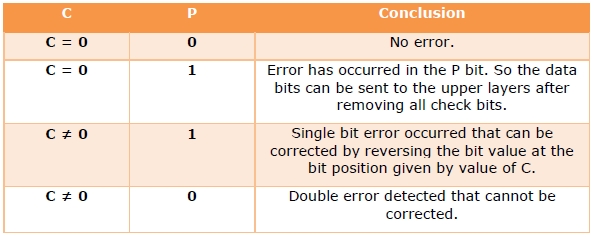
The decimal equivalent of the parity bits binary values is calculated. If it is 0, there is no error. Otherwise, the decimal value gives the bit position which has error. For example, if c1c2c3c4 = 1001, it implies that the data bit at position 9, decimal equivalent of 1001, has error. The bit is flipped (converted from 0 to 1 or vice versa) to get the correct message.
Example 4 − Suppose that an incoming message 11110101101 is received.
Step 1 − At first the number of redundant bits are calculated using the formula 2r ≥ m + r + 1. Here, m + r + 1 = 11 + 1 = 12. The minimum value of r such that 2r ≥ 12 is 4.
Step 2 − The redundant bits are positioned as below −
Step 3 − Even parity checking is done −
c1 = even_parity(1, 3, 5, 7, 9, 11) = 0
c2 = even_parity(2, 3, 6, 7, 10, 11) = 0
c3 = even_parity (4, 5, 6, 7) = 0
c4 = even_parity (8, 9, 10, 11) = 0
Step 4 – Since the value of the check bits c1c2c3c4 = 0000 = 0, there are no errors in this message.
Hamming Code for double error detection
The Hamming code can be modified to correct a single error and detect double errors by adding a parity bit as the MSB, which is the XOR of all other bits.
Example 5 − If we consider the codeword, 11000101100, sent as in example 3, after adding P = XOR(1,1,0,0,0,1,0,1,1,0,0) = 0, the new codeword to be sent will be 011000101100.
At the receiver’s end, error detection is done as shown in the following table −
Пример
. Предположим, в канале связи под действием
помех произошло искажение и вместо
0100101 было принято 01001(1)1.
Решение:
Для обнаружения ошибки производят уже
знакомые нам проверки на четность.
Первая
проверка:
сумма П1+П3+П5+П7
= 0+0+1+1 четна.
В младший разряд номера ошибочной
позиции запишем 0.
Вторая
проверка:
сумма П2+П3+П6+П7
= 1+0+1+1 нечетна.
Во второй разряд номера ошибочной
позиции запишем 1
Третья
проверка:
сумма П4+П5+П6+П7
= 0+1+1+1 нечетна.
В третий разряд номера ошибочной позиции
запишем 1. Номер ошибочной позиции 110=
6. Следовательно,
символ шестой позиции следует изменить
на обратный, и получим правильную кодовую
комбинацию.
Код, исправляющий
одиночную и обнаруживающий двойную
ошибки
Если по изложенным
выше правилам строить корректирующий
код с обнаружением и исправлением
одиночной ошибки для равномерного
двоичного кода, то первые 16 кодовых
комбинаций будут иметь вид, показанный
в таблице. Такой код может быть использован
для построения кода с исправлением
одиночной ошибки и обнаружением двойной.
Для
этого, кроме указанных выше проверок
по контрольным позициям, следует провести
еще одну проверку на четность для всей
строки в целом. Чтобы осуществить такую
проверку, следует к каждой строке кода
добавить контрольные символы, записанные
в дополнительной колонке (таблица,
колонка 8). Тогда в случае одной ошибки
проверки по позициям укажут номер
ошибочной позиции, а проверка на четность
— на наличие ошибки. Если проверки позиций
укажут на наличие ошибки, а проверка на
четность не фиксирует ее, значит в
кодовой комбинации две ошибки.
Лекция 8
8.1 Двоичные циклические коды
Вышеприведенная
процедура построения линейного кода
матричным методом имеет ряд недостатков.
Она неоднозначна (МДР можно задать
различным образом) и неудобна
в реализации в виде технических устройств.
Этих недостатков лишены
линейные корректирующие коды, принадлежащие
к классу циклических.
Циклическими
называют
линейные (n,k)-коды,
обладающие
следующим свойством:
для любого кодового слова:
![]()
существует другое
кодовое слово:
![]()
полученное
циклическим сдвигом элементов исходного
кодового слова ||КС||
вправо
или влево, которое также принадлежит
этому коду.
Для
описания циклических кодов используют
полиномы с фиктивной переменной
X.
Например,
пусть кодовое слово ||КС||
=
||011010||.
Его
можно описать полиномом
![]()
Таким
образом, разряды кодового слова в
описывающем его полиноме используются
в качестве коэффициентов при степенях
фиктивной переменной
X.
Наибольшая
степень фиктивной переменной X
в
слагаемом с ненулевым
коэффициентом называется степенью
полинома. В вышеприведенном примере
получился полином 4-й степени.
Теперь
действия над кодовыми словами сводятся
к действиям над полиномами.
Вместо алгебры матриц здесь используется
алгебра полиномов.
Рассмотрим
алгебраические действия над полиномами,
используемые в теории
циклических кодов. Суммирование
полиномов разберем на примере
С(Х)=А(Х)+В(Х).
Пусть
||A||
= ||011010||,
||В|| =
||110111|.
Тогда
![]()
![]()
![]()
—————————————————————
![]()
Таким
образом, при суммировании коэффициентов
при X
в одинаковой степени
результат берется по модулю 2. При таком
правиле вычитание эквивалентно
суммированию.
Умножение
выполняется как обычно, но с использованием
суммирования
по модулю 2.
Рассмотрим
умножение на примере умножения полинома
(X3+X1+X0)
на
полином X1+X0
X3
+ 0*X2+X1+X0
*
X1+X0
—————————————————
X3+
0*X2+X1+Х0
X4+0*Х3+
X2+Х1
____________________________________
Х4+
X3+
X2+0*X1+X0
Операция
— обратная умножению -деление. Деление
полиномов выполняется как обычно, за
исключением того, что вычитание
выполняется по модулю 2. Вспомним, что
вычитание по модулю 2 эквивалентно
сложению по модулю 2
Пример
деления полинома X6+X4+X3
на полином
X3+X2+1
X6+0*X5+X4
+ X3+0*X2+0*X1+0
| X3+X2+1
X6+X5+0*X4+X3 результат== |X3+X2
————————————
X5
+X4
+ 0*X3+0*X2
X5
+X4
+ 0*X3+
X2
—————————————-
остаток==
X2
=
100
Циклический
сдвиг влево на одну позицию коэффициентов
полинома степени n-1
получается
путем его умножения на X
с
последующим вычитанием из
результата полинома Xn+1,
если его порядок >
п.
Проверим это на
примере.
Пусть требуется
выполнить циклический сдвиг влево на
одну позицию
коэффициентов
полинома
C(X)=X5+Х3+X2+1
→ (101101)
В результате должен
получиться полином
C1(X)=X4+Х3+X1+1
→ (011011)
Это легко
доказывается:
C1(X)=C(X)*X-(X6+1)=(X6+Х4+X3+X)+(
X6+1)=X4+Х3+X1+1
В
основе циклического кода лежит образующий
полином r-го
порядка
(напомним, что r—
число дополнительных разрядов). Будем
обозначать
его gr(X).
Образование
кодовых слов (кодирование) КС
выполняется
путем умножения
информационного полинома с коэффициентами,
являющимися информационной
последовательностью
И(Х)
порядка
i<k
на
образующий полином gr(X)
КСr+k(Х)=gr(X)+ИСk(Х).
Принятое кодовое
слово может отличаться от переданного
искаженными разрядами в результате
воздействия помех.
ПКС(Х)=КС(Х)+ВО(Х).
где
ВО(Х)
— полином
вектора ошибки, а суммирование, как
обычно, ведется
по модулю 2.
Декодирование,
как и раньше начинается с нахождения
опознавателя,
в данном случае в виде полинома ОП(Х).
Этот
полином вычисляется как
остаток от деления полинома принятого
кодового слова ПКС(Х)
на
образующий
полином g(Х):
Первое
слагаемое остатка не имеет, т.к. кодовое
слово было образовано путем умножения
полинома информационной последовательности
на
образующий полином. Следовательно, и в
данном случае опознаватель
полностью зависит от вектора ошибки.
Образующий
полином выбирается таким, чтобы при
данном r
как
можно
большее число отношений ВО(Х)/g(Х)
давало
различные остатки.
Такому
требованию отвечают так называемые
неприводимые
полиномы,
которые
не делятся без остатка ни на один полином
степени r
и ниже, а
делятся только сами на себя и на 1.
Приведенная
здесь процедура образования кодового
слова неудобна тем,
что такой код получается несистематическим,
т.е. таким, в кодовых словах
которого нельзя выделить информационные
и дополнительные разряды.
Этот недостаток
был устранен следующим образом.
Способ
кодирования, приводящий к получению
систематического линейного циклического
кода, состоит в приписывании к
информационной
последовательности И
дополнительных разрядов ДР.
Эти
дополнительные разряды предлагается
находить по следующей формуле:
Порядок
полинома ДР(Х)
гарантировано
меньше r
(поскольку
это остаток).
Приписывание
дополнительных разрядов к информационной
последовательности,
используя алгебру полиномов, можно
описать формулой:
![]()
Одним
из свойств циклических линейных кодов
является то, что результат
деления любого разрешенного кодового
слова КС
на
образующий полином также, является
разрешенным кодовым словом.
Покажем,
что получаемые по вышеприведенному
алгоритму кодовые
слова являются кодовыми словами
циклического линейного кода. Для
этого нужно убедиться в том, что
произвольное разрешенное кодовое
слово делится на образующий полином
g(X)
без остатка:
Рассмотрим первое
слагаемое:
где
d(Х)
— целая
часть результата деления.
Подставим полученную
сумму на место первого слагаемого:
![]() Суммирование
Суммирование
последних двух слагаемых дает нулевой
результат (напомним,
что суммирование выполняется по модулю
2).
Значит
![]() —
—
целая часть деления. Остатка нет. Это
означает,
что описанный выше способ кодирования
соответствует циклическому
коду.
Соседние файлы в предмете [НЕСОРТИРОВАННОЕ]
- #
- #
- #
- #
- #
- #
- #
- #
- #
- #
- #
| Binary Hamming codes | |
|---|---|
|
The Hamming(7,4) code (with r = 3) |
|
| Named after | Richard W. Hamming |
| Classification | |
| Type | Linear block code |
| Block length | 2r − 1 where r ≥ 2 |
| Message length | 2r − r − 1 |
| Rate | 1 − r/(2r − 1) |
| Distance | 3 |
| Alphabet size | 2 |
| Notation | [2r − 1, 2r − r − 1, 3]2-code |
| Properties | |
| perfect code | |
|
In computer science and telecommunication, Hamming codes are a family of linear error-correcting codes. Hamming codes can detect one-bit and two-bit errors, or correct one-bit errors without detection of uncorrected errors. By contrast, the simple parity code cannot correct errors, and can detect only an odd number of bits in error. Hamming codes are perfect codes, that is, they achieve the highest possible rate for codes with their block length and minimum distance of three.[1]
Richard W. Hamming invented Hamming codes in 1950 as a way of automatically correcting errors introduced by punched card readers. In his original paper, Hamming elaborated his general idea, but specifically focused on the Hamming(7,4) code which adds three parity bits to four bits of data.[2]
In mathematical terms, Hamming codes are a class of binary linear code. For each integer r ≥ 2 there is a code-word with block length n = 2r − 1 and message length k = 2r − r − 1. Hence the rate of Hamming codes is R = k / n = 1 − r / (2r − 1), which is the highest possible for codes with minimum distance of three (i.e., the minimal number of bit changes needed to go from any code word to any other code word is three) and block length 2r − 1. The parity-check matrix of a Hamming code is constructed by listing all columns of length r that are non-zero, which means that the dual code of the Hamming code is the shortened Hadamard code. The parity-check matrix has the property that any two columns are pairwise linearly independent.
Due to the limited redundancy that Hamming codes add to the data, they can only detect and correct errors when the error rate is low. This is the case in computer memory (usually RAM), where bit errors are extremely rare and Hamming codes are widely used, and a RAM with this correction system is a ECC RAM (ECC memory). In this context, an extended Hamming code having one extra parity bit is often used. Extended Hamming codes achieve a Hamming distance of four, which allows the decoder to distinguish between when at most one one-bit error occurs and when any two-bit errors occur. In this sense, extended Hamming codes are single-error correcting and double-error detecting, abbreviated as SECDED.
History[edit]
Richard Hamming, the inventor of Hamming codes, worked at Bell Labs in the late 1940s on the Bell Model V computer, an electromechanical relay-based machine with cycle times in seconds. Input was fed in on punched paper tape, seven-eighths of an inch wide, which had up to six holes per row. During weekdays, when errors in the relays were detected, the machine would stop and flash lights so that the operators could correct the problem. During after-hours periods and on weekends, when there were no operators, the machine simply moved on to the next job.
Hamming worked on weekends, and grew increasingly frustrated with having to restart his programs from scratch due to detected errors. In a taped interview, Hamming said, «And so I said, ‘Damn it, if the machine can detect an error, why can’t it locate the position of the error and correct it?’».[3] Over the next few years, he worked on the problem of error-correction, developing an increasingly powerful array of algorithms. In 1950, he published what is now known as Hamming code, which remains in use today in applications such as ECC memory.
Codes predating Hamming[edit]
A number of simple error-detecting codes were used before Hamming codes, but none were as effective as Hamming codes in the same overhead of space.
Parity[edit]
Parity adds a single bit that indicates whether the number of ones (bit-positions with values of one) in the preceding data was even or odd. If an odd number of bits is changed in transmission, the message will change parity and the error can be detected at this point; however, the bit that changed may have been the parity bit itself. The most common convention is that a parity value of one indicates that there is an odd number of ones in the data, and a parity value of zero indicates that there is an even number of ones. If the number of bits changed is even, the check bit will be valid and the error will not be detected.
Moreover, parity does not indicate which bit contained the error, even when it can detect it. The data must be discarded entirely and re-transmitted from scratch. On a noisy transmission medium, a successful transmission could take a long time or may never occur. However, while the quality of parity checking is poor, since it uses only a single bit, this method results in the least overhead.
Two-out-of-five code[edit]
A two-out-of-five code is an encoding scheme which uses five bits consisting of exactly three 0s and two 1s. This provides ten possible combinations, enough to represent the digits 0–9. This scheme can detect all single bit-errors, all odd numbered bit-errors and some even numbered bit-errors (for example the flipping of both 1-bits). However it still cannot correct any of these errors.
Repetition[edit]
Another code in use at the time repeated every data bit multiple times in order to ensure that it was sent correctly. For instance, if the data bit to be sent is a 1, an n = 3 repetition code will send 111. If the three bits received are not identical, an error occurred during transmission. If the channel is clean enough, most of the time only one bit will change in each triple. Therefore, 001, 010, and 100 each correspond to a 0 bit, while 110, 101, and 011 correspond to a 1 bit, with the greater quantity of digits that are the same (‘0’ or a ‘1’) indicating what the data bit should be. A code with this ability to reconstruct the original message in the presence of errors is known as an error-correcting code. This triple repetition code is a Hamming code with m = 2, since there are two parity bits, and 22 − 2 − 1 = 1 data bit.
Such codes cannot correctly repair all errors, however. In our example, if the channel flips two bits and the receiver gets 001, the system will detect the error, but conclude that the original bit is 0, which is incorrect. If we increase the size of the bit string to four, we can detect all two-bit errors but cannot correct them (the quantity of parity bits is even); at five bits, we can both detect and correct all two-bit errors, but not all three-bit errors.
Moreover, increasing the size of the parity bit string is inefficient, reducing throughput by three times in our original case, and the efficiency drops drastically as we increase the number of times each bit is duplicated in order to detect and correct more errors.
Description[edit]
If more error-correcting bits are included with a message, and if those bits can be arranged such that different incorrect bits produce different error results, then bad bits could be identified. In a seven-bit message, there are seven possible single bit errors, so three error control bits could potentially specify not only that an error occurred but also which bit caused the error.
Hamming studied the existing coding schemes, including two-of-five, and generalized their concepts. To start with, he developed a nomenclature to describe the system, including the number of data bits and error-correction bits in a block. For instance, parity includes a single bit for any data word, so assuming ASCII words with seven bits, Hamming described this as an (8,7) code, with eight bits in total, of which seven are data. The repetition example would be (3,1), following the same logic. The code rate is the second number divided by the first, for our repetition example, 1/3.
Hamming also noticed the problems with flipping two or more bits, and described this as the «distance» (it is now called the Hamming distance, after him). Parity has a distance of 2, so one bit flip can be detected but not corrected, and any two bit flips will be invisible. The (3,1) repetition has a distance of 3, as three bits need to be flipped in the same triple to obtain another code word with no visible errors. It can correct one-bit errors or it can detect — but not correct — two-bit errors. A (4,1) repetition (each bit is repeated four times) has a distance of 4, so flipping three bits can be detected, but not corrected. When three bits flip in the same group there can be situations where attempting to correct will produce the wrong code word. In general, a code with distance k can detect but not correct k − 1 errors.
Hamming was interested in two problems at once: increasing the distance as much as possible, while at the same time increasing the code rate as much as possible. During the 1940s he developed several encoding schemes that were dramatic improvements on existing codes. The key to all of his systems was to have the parity bits overlap, such that they managed to check each other as well as the data.
General algorithm[edit]
The following general algorithm generates a single-error correcting (SEC) code for any number of bits. The main idea is to choose the error-correcting bits such that the index-XOR (the XOR of all the bit positions containing a 1) is 0. We use positions 1, 10, 100, etc. (in binary) as the error-correcting bits, which guarantees it is possible to set the error-correcting bits so that the index-XOR of the whole message is 0. If the receiver receives a string with index-XOR 0, they can conclude there were no corruptions, and otherwise, the index-XOR indicates the index of the corrupted bit.
An algorithm can be deduced from the following description:
- Number the bits starting from 1: bit 1, 2, 3, 4, 5, 6, 7, etc.
- Write the bit numbers in binary: 1, 10, 11, 100, 101, 110, 111, etc.
- All bit positions that are powers of two (have a single 1 bit in the binary form of their position) are parity bits: 1, 2, 4, 8, etc. (1, 10, 100, 1000)
- All other bit positions, with two or more 1 bits in the binary form of their position, are data bits.
- Each data bit is included in a unique set of 2 or more parity bits, as determined by the binary form of its bit position.
- Parity bit 1 covers all bit positions which have the least significant bit set: bit 1 (the parity bit itself), 3, 5, 7, 9, etc.
- Parity bit 2 covers all bit positions which have the second least significant bit set: bits 2-3, 6-7, 10-11, etc.
- Parity bit 4 covers all bit positions which have the third least significant bit set: bits 4–7, 12–15, 20–23, etc.
- Parity bit 8 covers all bit positions which have the fourth least significant bit set: bits 8–15, 24–31, 40–47, etc.
- In general each parity bit covers all bits where the bitwise AND of the parity position and the bit position is non-zero.
If a byte of data to be encoded is 10011010, then the data word (using _ to represent the parity bits) would be __1_001_1010, and the code word is 011100101010.
The choice of the parity, even or odd, is irrelevant but the same choice must be used for both encoding and decoding.
This general rule can be shown visually:
-
Bit position 1 2 3 4 5 6 7 8 9 10 11 12 13 14 15 16 17 18 19 20 … Encoded data bits p1 p2 d1 p4 d2 d3 d4 p8 d5 d6 d7 d8 d9 d10 d11 p16 d12 d13 d14 d15 Parity
bit
coveragep1 
p2 p4
p8 p16
Shown are only 20 encoded bits (5 parity, 15 data) but the pattern continues indefinitely. The key thing about Hamming Codes that can be seen from visual inspection is that any given bit is included in a unique set of parity bits. To check for errors, check all of the parity bits. The pattern of errors, called the error syndrome, identifies the bit in error. If all parity bits are correct, there is no error. Otherwise, the sum of the positions of the erroneous parity bits identifies the erroneous bit. For example, if the parity bits in positions 1, 2 and 8 indicate an error, then bit 1+2+8=11 is in error. If only one parity bit indicates an error, the parity bit itself is in error.
With m parity bits, bits from 1 up to 

| Parity bits | Total bits | Data bits | Name | Rate |
|---|---|---|---|---|
| 2 | 3 | 1 | Hamming(3,1) (Triple repetition code) |
1/3 ≈ 0.333 |
| 3 | 7 | 4 | Hamming(7,4) | 4/7 ≈ 0.571 |
| 4 | 15 | 11 | Hamming(15,11) | 11/15 ≈ 0.733 |
| 5 | 31 | 26 | Hamming(31,26) | 26/31 ≈ 0.839 |
| 6 | 63 | 57 | Hamming(63,57) | 57/63 ≈ 0.905 |
| 7 | 127 | 120 | Hamming(127,120) | 120/127 ≈ 0.945 |
| 8 | 255 | 247 | Hamming(255,247) | 247/255 ≈ 0.969 |
| … | ||||
| m |  |
 |
Hamming |

|
Hamming codes with additional parity (SECDED)[edit]
Hamming codes have a minimum distance of 3, which means that the decoder can detect and correct a single error, but it cannot distinguish a double bit error of some codeword from a single bit error of a different codeword. Thus, some double-bit errors will be incorrectly decoded as if they were single bit errors and therefore go undetected, unless no correction is attempted.
To remedy this shortcoming, Hamming codes can be extended by an extra parity bit. This way, it is possible to increase the minimum distance of the Hamming code to 4, which allows the decoder to distinguish between single bit errors and two-bit errors. Thus the decoder can detect and correct a single error and at the same time detect (but not correct) a double error.
If the decoder does not attempt to correct errors, it can reliably detect triple bit errors. If the decoder does correct errors, some triple errors will be mistaken for single errors and «corrected» to the wrong value. Error correction is therefore a trade-off between certainty (the ability to reliably detect triple bit errors) and resiliency (the ability to keep functioning in the face of single bit errors).
This extended Hamming code was popular in computer memory systems, starting with IBM 7030 Stretch in 1961,[4] where it is known as SECDED (or SEC-DED, abbreviated from single error correction, double error detection).[5] Server computers in 21st century, while typically keeping the SECDED level of protection, no longer use the Hamming’s method, relying instead on the designs with longer codewords (128 to 256 bits of data) and modified balanced parity-check trees.[4] The (72,64) Hamming code is still popular in some hardware designs, including Xilinx FPGA families.[4]
[7,4] Hamming code[edit]

Graphical depiction of the four data bits and three parity bits and which parity bits apply to which data bits
In 1950, Hamming introduced the [7,4] Hamming code. It encodes four data bits into seven bits by adding three parity bits. It can detect and correct single-bit errors. With the addition of an overall parity bit, it can also detect (but not correct) double-bit errors.
Construction of G and H[edit]
The matrix

and 
This is the construction of G and H in standard (or systematic) form. Regardless of form, G and H for linear block codes must satisfy

Since [7, 4, 3] = [n, k, d] = [2m − 1, 2m − 1 − m, 3]. The parity-check matrix H of a Hamming code is constructed by listing all columns of length m that are pair-wise independent.
Thus H is a matrix whose left side is all of the nonzero n-tuples where order of the n-tuples in the columns of matrix does not matter. The right hand side is just the (n − k)-identity matrix.
So G can be obtained from H by taking the transpose of the left hand side of H with the identity k-identity matrix on the left hand side of G.
The code generator matrix 


and

Finally, these matrices can be mutated into equivalent non-systematic codes by the following operations:[6]
- Column permutations (swapping columns)
- Elementary row operations (replacing a row with a linear combination of rows)
Encoding[edit]
- Example
From the above matrix we have 2k = 24 = 16 codewords.
Let 
![{displaystyle {vec {a}}=[a_{1},a_{2},a_{3},a_{4}],quad a_{i}in {0,1}}](https://wikimedia.org/api/rest_v1/media/math/render/svg/898ddf319567d4af0acecf5c7fd450f5f466e28b)


For example, let ![{displaystyle {vec {a}}=[1,0,1,1]}](https://wikimedia.org/api/rest_v1/media/math/render/svg/e838e2ec81e9fe6223596b61f747b195d3d338fb)


[7,4] Hamming code with an additional parity bit[edit]

The same [7,4] example from above with an extra parity bit. This diagram is not meant to correspond to the matrix H for this example.
The [7,4] Hamming code can easily be extended to an [8,4] code by adding an extra parity bit on top of the (7,4) encoded word (see Hamming(7,4)).
This can be summed up with the revised matrices:

and

Note that H is not in standard form. To obtain G, elementary row operations can be used to obtain an equivalent matrix to H in systematic form:

For example, the first row in this matrix is the sum of the second and third rows of H in non-systematic form. Using the systematic construction for Hamming codes from above, the matrix A is apparent and the systematic form of G is written as

The non-systematic form of G can be row reduced (using elementary row operations) to match this matrix.
The addition of the fourth row effectively computes the sum of all the codeword bits (data and parity) as the fourth parity bit.
For example, 1011 is encoded (using the non-systematic form of G at the start of this section) into 01100110 where blue digits are data; red digits are parity bits from the [7,4] Hamming code; and the green digit is the parity bit added by the [8,4] code.
The green digit makes the parity of the [7,4] codewords even.
Finally, it can be shown that the minimum distance has increased from 3, in the [7,4] code, to 4 in the [8,4] code. Therefore, the code can be defined as [8,4] Hamming code.
To decode the [8,4] Hamming code, first check the parity bit. If the parity bit indicates an error, single error correction (the [7,4] Hamming code) will indicate the error location, with «no error» indicating the parity bit. If the parity bit is correct, then single error correction will indicate the (bitwise) exclusive-or of two error locations. If the locations are equal («no error») then a double bit error either has not occurred, or has cancelled itself out. Otherwise, a double bit error has occurred.
See also[edit]
- Coding theory
- Golay code
- Reed–Muller code
- Reed–Solomon error correction
- Turbo code
- Low-density parity-check code
- Hamming bound
- Hamming distance
Notes[edit]
- ^ See Lemma 12 of
- ^ Hamming (1950), pp. 153–154.
- ^ Thompson, Thomas M. (1983), From Error-Correcting Codes through Sphere Packings to Simple Groups, The Carus Mathematical Monographs (#21), Mathematical Association of America, pp. 16–17, ISBN 0-88385-023-0
- ^ a b c Kythe & Kythe 2017, p. 115.
- ^ Kythe & Kythe 2017, p. 95.
- ^ a b Moon T. Error correction coding: Mathematical Methods and
Algorithms. John Wiley and Sons, 2005.(Cap. 3) ISBN 978-0-471-64800-0
References[edit]
- Hamming, Richard Wesley (1950). «Error detecting and error correcting codes» (PDF). Bell System Technical Journal. 29 (2): 147–160. doi:10.1002/j.1538-7305.1950.tb00463.x. S2CID 61141773. Archived (PDF) from the original on 2022-10-09.
- Moon, Todd K. (2005). Error Correction Coding. New Jersey: John Wiley & Sons. ISBN 978-0-471-64800-0.
- MacKay, David J.C. (September 2003). Information Theory, Inference and Learning Algorithms. Cambridge: Cambridge University Press. ISBN 0-521-64298-1.
- D.K. Bhattacharryya, S. Nandi. «An efficient class of SEC-DED-AUED codes». 1997 International Symposium on Parallel Architectures, Algorithms and Networks (ISPAN ’97). pp. 410–415. doi:10.1109/ISPAN.1997.645128.
- «Mathematical Challenge April 2013 Error-correcting codes» (PDF). swissQuant Group Leadership Team. April 2013. Archived (PDF) from the original on 2017-09-12.
- Kythe, Dave K.; Kythe, Prem K. (28 July 2017). «Extended Hamming Codes». Algebraic and Stochastic Coding Theory. CRC Press. pp. 95–116. ISBN 978-1-351-83245-8.
External links[edit]
- Visual Explanation of Hamming Codes
- CGI script for calculating Hamming distances (from R. Tervo, UNB, Canada)
- Tool for calculating Hamming code
| Binary Hamming codes | |
|---|---|
|
The Hamming(7,4) code (with r = 3) |
|
| Named after | Richard W. Hamming |
| Classification | |
| Type | Linear block code |
| Block length | 2r − 1 where r ≥ 2 |
| Message length | 2r − r − 1 |
| Rate | 1 − r/(2r − 1) |
| Distance | 3 |
| Alphabet size | 2 |
| Notation | [2r − 1, 2r − r − 1, 3]2-code |
| Properties | |
| perfect code | |
|
In computer science and telecommunication, Hamming codes are a family of linear error-correcting codes. Hamming codes can detect one-bit and two-bit errors, or correct one-bit errors without detection of uncorrected errors. By contrast, the simple parity code cannot correct errors, and can detect only an odd number of bits in error. Hamming codes are perfect codes, that is, they achieve the highest possible rate for codes with their block length and minimum distance of three.[1]
Richard W. Hamming invented Hamming codes in 1950 as a way of automatically correcting errors introduced by punched card readers. In his original paper, Hamming elaborated his general idea, but specifically focused on the Hamming(7,4) code which adds three parity bits to four bits of data.[2]
In mathematical terms, Hamming codes are a class of binary linear code. For each integer r ≥ 2 there is a code-word with block length n = 2r − 1 and message length k = 2r − r − 1. Hence the rate of Hamming codes is R = k / n = 1 − r / (2r − 1), which is the highest possible for codes with minimum distance of three (i.e., the minimal number of bit changes needed to go from any code word to any other code word is three) and block length 2r − 1. The parity-check matrix of a Hamming code is constructed by listing all columns of length r that are non-zero, which means that the dual code of the Hamming code is the shortened Hadamard code. The parity-check matrix has the property that any two columns are pairwise linearly independent.
Due to the limited redundancy that Hamming codes add to the data, they can only detect and correct errors when the error rate is low. This is the case in computer memory (usually RAM), where bit errors are extremely rare and Hamming codes are widely used, and a RAM with this correction system is a ECC RAM (ECC memory). In this context, an extended Hamming code having one extra parity bit is often used. Extended Hamming codes achieve a Hamming distance of four, which allows the decoder to distinguish between when at most one one-bit error occurs and when any two-bit errors occur. In this sense, extended Hamming codes are single-error correcting and double-error detecting, abbreviated as SECDED.
History[edit]
Richard Hamming, the inventor of Hamming codes, worked at Bell Labs in the late 1940s on the Bell Model V computer, an electromechanical relay-based machine with cycle times in seconds. Input was fed in on punched paper tape, seven-eighths of an inch wide, which had up to six holes per row. During weekdays, when errors in the relays were detected, the machine would stop and flash lights so that the operators could correct the problem. During after-hours periods and on weekends, when there were no operators, the machine simply moved on to the next job.
Hamming worked on weekends, and grew increasingly frustrated with having to restart his programs from scratch due to detected errors. In a taped interview, Hamming said, «And so I said, ‘Damn it, if the machine can detect an error, why can’t it locate the position of the error and correct it?’».[3] Over the next few years, he worked on the problem of error-correction, developing an increasingly powerful array of algorithms. In 1950, he published what is now known as Hamming code, which remains in use today in applications such as ECC memory.
Codes predating Hamming[edit]
A number of simple error-detecting codes were used before Hamming codes, but none were as effective as Hamming codes in the same overhead of space.
Parity[edit]
Parity adds a single bit that indicates whether the number of ones (bit-positions with values of one) in the preceding data was even or odd. If an odd number of bits is changed in transmission, the message will change parity and the error can be detected at this point; however, the bit that changed may have been the parity bit itself. The most common convention is that a parity value of one indicates that there is an odd number of ones in the data, and a parity value of zero indicates that there is an even number of ones. If the number of bits changed is even, the check bit will be valid and the error will not be detected.
Moreover, parity does not indicate which bit contained the error, even when it can detect it. The data must be discarded entirely and re-transmitted from scratch. On a noisy transmission medium, a successful transmission could take a long time or may never occur. However, while the quality of parity checking is poor, since it uses only a single bit, this method results in the least overhead.
Two-out-of-five code[edit]
A two-out-of-five code is an encoding scheme which uses five bits consisting of exactly three 0s and two 1s. This provides ten possible combinations, enough to represent the digits 0–9. This scheme can detect all single bit-errors, all odd numbered bit-errors and some even numbered bit-errors (for example the flipping of both 1-bits). However it still cannot correct any of these errors.
Repetition[edit]
Another code in use at the time repeated every data bit multiple times in order to ensure that it was sent correctly. For instance, if the data bit to be sent is a 1, an n = 3 repetition code will send 111. If the three bits received are not identical, an error occurred during transmission. If the channel is clean enough, most of the time only one bit will change in each triple. Therefore, 001, 010, and 100 each correspond to a 0 bit, while 110, 101, and 011 correspond to a 1 bit, with the greater quantity of digits that are the same (‘0’ or a ‘1’) indicating what the data bit should be. A code with this ability to reconstruct the original message in the presence of errors is known as an error-correcting code. This triple repetition code is a Hamming code with m = 2, since there are two parity bits, and 22 − 2 − 1 = 1 data bit.
Such codes cannot correctly repair all errors, however. In our example, if the channel flips two bits and the receiver gets 001, the system will detect the error, but conclude that the original bit is 0, which is incorrect. If we increase the size of the bit string to four, we can detect all two-bit errors but cannot correct them (the quantity of parity bits is even); at five bits, we can both detect and correct all two-bit errors, but not all three-bit errors.
Moreover, increasing the size of the parity bit string is inefficient, reducing throughput by three times in our original case, and the efficiency drops drastically as we increase the number of times each bit is duplicated in order to detect and correct more errors.
Description[edit]
If more error-correcting bits are included with a message, and if those bits can be arranged such that different incorrect bits produce different error results, then bad bits could be identified. In a seven-bit message, there are seven possible single bit errors, so three error control bits could potentially specify not only that an error occurred but also which bit caused the error.
Hamming studied the existing coding schemes, including two-of-five, and generalized their concepts. To start with, he developed a nomenclature to describe the system, including the number of data bits and error-correction bits in a block. For instance, parity includes a single bit for any data word, so assuming ASCII words with seven bits, Hamming described this as an (8,7) code, with eight bits in total, of which seven are data. The repetition example would be (3,1), following the same logic. The code rate is the second number divided by the first, for our repetition example, 1/3.
Hamming also noticed the problems with flipping two or more bits, and described this as the «distance» (it is now called the Hamming distance, after him). Parity has a distance of 2, so one bit flip can be detected but not corrected, and any two bit flips will be invisible. The (3,1) repetition has a distance of 3, as three bits need to be flipped in the same triple to obtain another code word with no visible errors. It can correct one-bit errors or it can detect — but not correct — two-bit errors. A (4,1) repetition (each bit is repeated four times) has a distance of 4, so flipping three bits can be detected, but not corrected. When three bits flip in the same group there can be situations where attempting to correct will produce the wrong code word. In general, a code with distance k can detect but not correct k − 1 errors.
Hamming was interested in two problems at once: increasing the distance as much as possible, while at the same time increasing the code rate as much as possible. During the 1940s he developed several encoding schemes that were dramatic improvements on existing codes. The key to all of his systems was to have the parity bits overlap, such that they managed to check each other as well as the data.
General algorithm[edit]
The following general algorithm generates a single-error correcting (SEC) code for any number of bits. The main idea is to choose the error-correcting bits such that the index-XOR (the XOR of all the bit positions containing a 1) is 0. We use positions 1, 10, 100, etc. (in binary) as the error-correcting bits, which guarantees it is possible to set the error-correcting bits so that the index-XOR of the whole message is 0. If the receiver receives a string with index-XOR 0, they can conclude there were no corruptions, and otherwise, the index-XOR indicates the index of the corrupted bit.
An algorithm can be deduced from the following description:
- Number the bits starting from 1: bit 1, 2, 3, 4, 5, 6, 7, etc.
- Write the bit numbers in binary: 1, 10, 11, 100, 101, 110, 111, etc.
- All bit positions that are powers of two (have a single 1 bit in the binary form of their position) are parity bits: 1, 2, 4, 8, etc. (1, 10, 100, 1000)
- All other bit positions, with two or more 1 bits in the binary form of their position, are data bits.
- Each data bit is included in a unique set of 2 or more parity bits, as determined by the binary form of its bit position.
- Parity bit 1 covers all bit positions which have the least significant bit set: bit 1 (the parity bit itself), 3, 5, 7, 9, etc.
- Parity bit 2 covers all bit positions which have the second least significant bit set: bits 2-3, 6-7, 10-11, etc.
- Parity bit 4 covers all bit positions which have the third least significant bit set: bits 4–7, 12–15, 20–23, etc.
- Parity bit 8 covers all bit positions which have the fourth least significant bit set: bits 8–15, 24–31, 40–47, etc.
- In general each parity bit covers all bits where the bitwise AND of the parity position and the bit position is non-zero.
If a byte of data to be encoded is 10011010, then the data word (using _ to represent the parity bits) would be __1_001_1010, and the code word is 011100101010.
The choice of the parity, even or odd, is irrelevant but the same choice must be used for both encoding and decoding.
This general rule can be shown visually:
-
Bit position 1 2 3 4 5 6 7 8 9 10 11 12 13 14 15 16 17 18 19 20 … Encoded data bits p1 p2 d1 p4 d2 d3 d4 p8 d5 d6 d7 d8 d9 d10 d11 p16 d12 d13 d14 d15 Parity
bit
coveragep1 p2 p4
p8 p16
Shown are only 20 encoded bits (5 parity, 15 data) but the pattern continues indefinitely. The key thing about Hamming Codes that can be seen from visual inspection is that any given bit is included in a unique set of parity bits. To check for errors, check all of the parity bits. The pattern of errors, called the error syndrome, identifies the bit in error. If all parity bits are correct, there is no error. Otherwise, the sum of the positions of the erroneous parity bits identifies the erroneous bit. For example, if the parity bits in positions 1, 2 and 8 indicate an error, then bit 1+2+8=11 is in error. If only one parity bit indicates an error, the parity bit itself is in error.
With m parity bits, bits from 1 up to
| Parity bits | Total bits | Data bits | Name | Rate |
|---|---|---|---|---|
| 2 | 3 | 1 | Hamming(3,1) (Triple repetition code) |
1/3 ≈ 0.333 |
| 3 | 7 | 4 | Hamming(7,4) | 4/7 ≈ 0.571 |
| 4 | 15 | 11 | Hamming(15,11) | 11/15 ≈ 0.733 |
| 5 | 31 | 26 | Hamming(31,26) | 26/31 ≈ 0.839 |
| 6 | 63 | 57 | Hamming(63,57) | 57/63 ≈ 0.905 |
| 7 | 127 | 120 | Hamming(127,120) | 120/127 ≈ 0.945 |
| 8 | 255 | 247 | Hamming(255,247) | 247/255 ≈ 0.969 |
| … | ||||
| m | |
|
Hamming |
|
Hamming codes with additional parity (SECDED)[edit]
Hamming codes have a minimum distance of 3, which means that the decoder can detect and correct a single error, but it cannot distinguish a double bit error of some codeword from a single bit error of a different codeword. Thus, some double-bit errors will be incorrectly decoded as if they were single bit errors and therefore go undetected, unless no correction is attempted.
To remedy this shortcoming, Hamming codes can be extended by an extra parity bit. This way, it is possible to increase the minimum distance of the Hamming code to 4, which allows the decoder to distinguish between single bit errors and two-bit errors. Thus the decoder can detect and correct a single error and at the same time detect (but not correct) a double error.
If the decoder does not attempt to correct errors, it can reliably detect triple bit errors. If the decoder does correct errors, some triple errors will be mistaken for single errors and «corrected» to the wrong value. Error correction is therefore a trade-off between certainty (the ability to reliably detect triple bit errors) and resiliency (the ability to keep functioning in the face of single bit errors).
This extended Hamming code was popular in computer memory systems, starting with IBM 7030 Stretch in 1961,[4] where it is known as SECDED (or SEC-DED, abbreviated from single error correction, double error detection).[5] Server computers in 21st century, while typically keeping the SECDED level of protection, no longer use the Hamming’s method, relying instead on the designs with longer codewords (128 to 256 bits of data) and modified balanced parity-check trees.[4] The (72,64) Hamming code is still popular in some hardware designs, including Xilinx FPGA families.[4]
[7,4] Hamming code[edit]
Graphical depiction of the four data bits and three parity bits and which parity bits apply to which data bits
In 1950, Hamming introduced the [7,4] Hamming code. It encodes four data bits into seven bits by adding three parity bits. It can detect and correct single-bit errors. With the addition of an overall parity bit, it can also detect (but not correct) double-bit errors.
Construction of G and H[edit]
The matrix
and
This is the construction of G and H in standard (or systematic) form. Regardless of form, G and H for linear block codes must satisfy
Since [7, 4, 3] = [n, k, d] = [2m − 1, 2m − 1 − m, 3]. The parity-check matrix H of a Hamming code is constructed by listing all columns of length m that are pair-wise independent.
Thus H is a matrix whose left side is all of the nonzero n-tuples where order of the n-tuples in the columns of matrix does not matter. The right hand side is just the (n − k)-identity matrix.
So G can be obtained from H by taking the transpose of the left hand side of H with the identity k-identity matrix on the left hand side of G.
The code generator matrix
and
Finally, these matrices can be mutated into equivalent non-systematic codes by the following operations:[6]
- Column permutations (swapping columns)
- Elementary row operations (replacing a row with a linear combination of rows)
Encoding[edit]
- Example
From the above matrix we have 2k = 24 = 16 codewords.
Let
For example, let
[7,4] Hamming code with an additional parity bit[edit]
The same [7,4] example from above with an extra parity bit. This diagram is not meant to correspond to the matrix H for this example.
The [7,4] Hamming code can easily be extended to an [8,4] code by adding an extra parity bit on top of the (7,4) encoded word (see Hamming(7,4)).
This can be summed up with the revised matrices:
and
Note that H is not in standard form. To obtain G, elementary row operations can be used to obtain an equivalent matrix to H in systematic form:
For example, the first row in this matrix is the sum of the second and third rows of H in non-systematic form. Using the systematic construction for Hamming codes from above, the matrix A is apparent and the systematic form of G is written as
The non-systematic form of G can be row reduced (using elementary row operations) to match this matrix.
The addition of the fourth row effectively computes the sum of all the codeword bits (data and parity) as the fourth parity bit.
For example, 1011 is encoded (using the non-systematic form of G at the start of this section) into 01100110 where blue digits are data; red digits are parity bits from the [7,4] Hamming code; and the green digit is the parity bit added by the [8,4] code.
The green digit makes the parity of the [7,4] codewords even.
Finally, it can be shown that the minimum distance has increased from 3, in the [7,4] code, to 4 in the [8,4] code. Therefore, the code can be defined as [8,4] Hamming code.
To decode the [8,4] Hamming code, first check the parity bit. If the parity bit indicates an error, single error correction (the [7,4] Hamming code) will indicate the error location, with «no error» indicating the parity bit. If the parity bit is correct, then single error correction will indicate the (bitwise) exclusive-or of two error locations. If the locations are equal («no error») then a double bit error either has not occurred, or has cancelled itself out. Otherwise, a double bit error has occurred.
See also[edit]
- Coding theory
- Golay code
- Reed–Muller code
- Reed–Solomon error correction
- Turbo code
- Low-density parity-check code
- Hamming bound
- Hamming distance
Notes[edit]
- ^ See Lemma 12 of
- ^ Hamming (1950), pp. 153–154.
- ^ Thompson, Thomas M. (1983), From Error-Correcting Codes through Sphere Packings to Simple Groups, The Carus Mathematical Monographs (#21), Mathematical Association of America, pp. 16–17, ISBN 0-88385-023-0
- ^ a b c Kythe & Kythe 2017, p. 115.
- ^ Kythe & Kythe 2017, p. 95.
- ^ a b Moon T. Error correction coding: Mathematical Methods and
Algorithms. John Wiley and Sons, 2005.(Cap. 3) ISBN 978-0-471-64800-0
References[edit]
- Hamming, Richard Wesley (1950). «Error detecting and error correcting codes» (PDF). Bell System Technical Journal. 29 (2): 147–160. doi:10.1002/j.1538-7305.1950.tb00463.x. S2CID 61141773. Archived (PDF) from the original on 2022-10-09.
- Moon, Todd K. (2005). Error Correction Coding. New Jersey: John Wiley & Sons. ISBN 978-0-471-64800-0.
- MacKay, David J.C. (September 2003). Information Theory, Inference and Learning Algorithms. Cambridge: Cambridge University Press. ISBN 0-521-64298-1.
- D.K. Bhattacharryya, S. Nandi. «An efficient class of SEC-DED-AUED codes». 1997 International Symposium on Parallel Architectures, Algorithms and Networks (ISPAN ’97). pp. 410–415. doi:10.1109/ISPAN.1997.645128.
- «Mathematical Challenge April 2013 Error-correcting codes» (PDF). swissQuant Group Leadership Team. April 2013. Archived (PDF) from the original on 2017-09-12.
- Kythe, Dave K.; Kythe, Prem K. (28 July 2017). «Extended Hamming Codes». Algebraic and Stochastic Coding Theory. CRC Press. pp. 95–116. ISBN 978-1-351-83245-8.
External links[edit]
- Visual Explanation of Hamming Codes
- CGI script for calculating Hamming distances (from R. Tervo, UNB, Canada)
- Tool for calculating Hamming code
Код Хэмминга
Содержание
- Самокорректирующийся код
- Алгоритм кодирования
- Самокорректирующийся код
- Результат работы программы
- Полученный мною опыт
Самокорректирующийся код
Код Хэ́мминга — наиболее известный из первых самоконтролирующихся и самокорректирующихся кодов. Построен применительно к двоичной системе счисления. Позволяет исправлять одиночную ошибку (ошибка в одном бите) и находить двойную.
Алгоритм кодирования
Предположим, что нужно сгенерировать код Хемминга для некоторого информационного кодового слова. В качестве примера возьмём 15-битовое кодовое слово x1…x15, хотя алгоритм пригоден для кодовых слов любой длины. В приведённой ниже таблице в первой строке даны номера позиций в кодовом слове, во второй — условное обозначение битов, в третьей — значения битов.
| 1 | 2 | 3 | 4 | 5 | 6 | 7 | 8 | 9 | 10 | 11 | 12 | 13 | 14 | 15 |
| x1 | x2 | x3 | x4 | x5 | x6 | x7 | x8 | x9 | x10 | x11 | x12 | x13 | x14 | x15 |
| 1 | 0 | 0 | 1 | 0 | 0 | 1 | 0 | 1 | 1 | 1 | 0 | 0 | 0 | 1 |
Вставим в информационное слово контрольные биты r0…r4 таким образом, чтобы номера их позиций представляли собой целые степени двойки: 1, 2, 4, 8, 16… Получим 20-разрядное слово с 15 информационными и 5 контрольными битами. Первоначально контрольные биты устанавливаем равными нулю. На рисунке контрольные биты выделены розовым цветом.
| 1 | 2 | 3 | 4 | 5 | 6 | 7 | 8 | 9 | 10 | 11 | 12 | 13 | 14 | 15 | 16 | 17 | 18 | 19 | 20 |
| r0 | r1 | x1 | r2 | x2 | x3 | x4 | r3 | x5 | x6 | x7 | x8 | x9 | x10 | x11 | r4 | x12 | x13 | x14 | x15 |
| 0 | 0 | 1 | 0 | 0 | 0 | 1 | 0 | 0 | 0 | 1 | 0 | 1 | 1 | 1 | 0 | 0 | 0 | 0 | 1 |
В общем случае количество контрольных бит в кодовом слове равно двоичному логарифму числа, на единицу большего, чем количество бит кодового слова (включая контрольные биты); логарифм округляется в большую сторону. Например, информационное слово длиной 1 бит требует двух контрольных разрядов, 2-, 3- или 4-битовое информационное слово — трёх, 5…11-битовое — четырёх, 12…26-битовое — пяти и т. д.
Добавим к таблице 5 строк (по количеству контрольных битов), в которые поместим матрицу преобразования. Каждая строка будет соответствовать одному контрольному биту (нулевой контрольный бит — верхняя строка, четвёртый — нижняя), каждый столбец — одному биту кодируемого слова. В каждом столбце матрицы преобразования поместим двоичный номер этого столбца, причём порядок следования битов будет обратный — младший бит расположим в верхней строке, старший — в нижней. Например, в третьем столбце матрицы будут стоять числа 11000, что соответствует двоичной записи числа три: 00011.
| 1 | 2 | 3 | 4 | 5 | 6 | 7 | 8 | 9 | 10 | 11 | 12 | 13 | 14 | 15 | 16 | 17 | 18 | 19 | 20 | ||
| r0 | r1 | x1 | r2 | x2 | x3 | x4 | r3 | x5 | x6 | x7 | x8 | x9 | x10 | x11 | r4 | x12 | x13 | x14 | x15 | ||
| 0 | 0 | 1 | 0 | 0 | 0 | 1 | 0 | 0 | 0 | 1 | 0 | 1 | 1 | 1 | 0 | 0 | 0 | 0 | 1 | ||
| 1 | 0 | 1 | 0 | 1 | 0 | 1 | 0 | 1 | 0 | 1 | 0 | 1 | 0 | 1 | 0 | 1 | 0 | 1 | 0 | r0 | |
| 0 | 1 | 1 | 0 | 0 | 1 | 1 | 0 | 0 | 1 | 1 | 0 | 0 | 1 | 1 | 0 | 0 | 1 | 1 | 0 | r1 | |
| 0 | 0 | 0 | 1 | 1 | 1 | 1 | 0 | 0 | 0 | 0 | 1 | 1 | 1 | 1 | 0 | 0 | 0 | 0 | 1 | r2 | |
| 0 | 0 | 0 | 0 | 0 | 0 | 0 | 1 | 1 | 1 | 1 | 1 | 1 | 1 | 1 | 0 | 0 | 0 | 0 | 0 | r3 | |
| 0 | 0 | 0 | 0 | 0 | 0 | 0 | 0 | 0 | 0 | 0 | 0 | 0 | 0 | 0 | 1 | 1 | 1 | 1 | 1 | r4 |
В правой части таблицы мы оставили пустым один столбец, в который поместим результаты вычислений контрольных битов. Вычисление контрольных битов производим следующим образом. Берём одну из строк матрицы преобразования (например, r0) и находим её скалярное произведение с кодовым словом, то есть перемножаем соответствующие биты обеих строк и находим сумму произведений. Если сумма получилась больше единицы, находим остаток от его деления на 2. Иными словами, мы подсчитываем сколько раз в кодовом слове и соответствующей строке матрицы в одинаковых позициях стоят единицы и берём это число по модулю 2.
Если описывать этот процесс в терминах матричной алгебры, то операция представляет собой перемножение матрицы преобразования на матрицу-столбец кодового слова, в результате чего получается матрица-столбец контрольных разрядов, которые нужно взять по модулю 2.
Например, для строки r0:
r0 = (1·0+0·0+1·1+0·0+1·0+0·0+1·1+0·0+1·0+0·0+1·1+0·0+1·1+0·1+1·1+0·0+1·0+0·0+1·0+0·1) mod 2 = 5 mod 2 = 1.
Полученные контрольные биты вставляем в кодовое слово вместо стоявших там ранее нулей. По аналогии находим проверочные биты в остальных строках. Кодирование по Хэммингу завершено. Полученное кодовое слово — 11110010001011110001.
| 1 | 2 | 3 | 4 | 5 | 6 | 7 | 8 | 9 | 10 | 11 | 12 | 13 | 14 | 15 | 16 | 17 | 18 | 19 | 20 | ||
| r0 | r1 | x1 | r2 | x2 | x3 | x4 | r3 | x5 | x6 | x7 | x8 | x9 | x10 | x11 | r4 | x12 | x13 | x14 | x15 | ||
| 0 | 0 | 1 | 0 | 0 | 0 | 1 | 0 | 0 | 0 | 1 | 0 | 1 | 1 | 1 | 0 | 0 | 0 | 0 | 1 | ||
| 1 | 0 | 1 | 0 | 1 | 0 | 1 | 0 | 1 | 0 | 1 | 0 | 1 | 0 | 1 | 0 | 1 | 0 | 1 | 0 | r0 | 1 |
| 0 | 1 | 1 | 0 | 0 | 1 | 1 | 0 | 0 | 1 | 1 | 0 | 0 | 1 | 1 | 0 | 0 | 1 | 1 | 0 | r1 | 1 |
| 0 | 0 | 0 | 1 | 1 | 1 | 1 | 0 | 0 | 0 | 0 | 1 | 1 | 1 | 1 | 0 | 0 | 0 | 0 | 1 | r2 | 1 |
| 0 | 0 | 0 | 0 | 0 | 0 | 0 | 1 | 1 | 1 | 1 | 1 | 1 | 1 | 1 | 0 | 0 | 0 | 0 | 0 | r3 | 0 |
| 0 | 0 | 0 | 0 | 0 | 0 | 0 | 0 | 0 | 0 | 0 | 0 | 0 | 0 | 0 | 1 | 1 | 1 | 1 | 1 | r4 | 1 |
Алгоритм декодирования
Алгоритм декодирования по Хэммингу абсолютно идентичен алгоритму кодирования. Матрица преобразования соответствующей размерности умножается на матрицу-столбец кодового слова и каждый элемент полученной матрицы-столбца берётся по модулю 2. Полученная матрица-столбец получила название «матрица синдромов». Легко проверить, что кодовое слово, сформированное в соответствии с алгоритмом, описанным в предыдущем разделе, всегда даёт нулевую матрицу синдромов.
Матрица синдромов становится ненулевой, если в результате ошибки (например, при передаче слова по линии связи с шумами) один из битов исходного слова изменил своё значение. Предположим для примера, что в кодовом слове, полученном в предыдущем разделе, шестой бит изменил своё значение с нуля на единицу (на рисунке обозначено красным цветом). Тогда получим следующую матрицу синдромов.
| 1 | 2 | 3 | 4 | 5 | 6 | 7 | 8 | 9 | 10 | 11 | 12 | 13 | 14 | 15 | 16 | 17 | 18 | 19 | 20 | ||
|---|---|---|---|---|---|---|---|---|---|---|---|---|---|---|---|---|---|---|---|---|---|
| r0 | r1 | x1 | r2 | x2 | x3 | x4 | r3 | x5 | x6 | x7 | x8 | x9 | x10 | x11 | r4 | x12 | x13 | x14 | x15 | ||
| 1 | 1 | 1 | 1 | 0 | 1 | 1 | 0 | 0 | 0 | 1 | 0 | 1 | 1 | 1 | 1 | 0 | 0 | 0 | 1 | ||
| 1 | 0 | 1 | 0 | 1 | 0 | 1 | 0 | 1 | 0 | 1 | 0 | 1 | 0 | 1 | 0 | 1 | 0 | 1 | 0 | s0 | 0 |
| 0 | 1 | 1 | 0 | 0 | 1 | 1 | 0 | 0 | 1 | 1 | 0 | 0 | 1 | 1 | 0 | 0 | 1 | 1 | 0 | s1 | 1 |
| 0 | 0 | 0 | 1 | 1 | 1 | 1 | 0 | 0 | 0 | 0 | 1 | 1 | 1 | 1 | 0 | 0 | 0 | 0 | 1 | s2 | 1 |
| 0 | 0 | 0 | 0 | 0 | 0 | 0 | 1 | 1 | 1 | 1 | 1 | 1 | 1 | 1 | 0 | 0 | 0 | 0 | 0 | s3 | 0 |
| 0 | 0 | 0 | 0 | 0 | 0 | 0 | 0 | 0 | 0 | 0 | 0 | 0 | 0 | 0 | 1 | 1 | 1 | 1 | 1 | s4 | 0 |
Заметим, что при однократной ошибке матрица синдромов всегда представляет собой двоичную запись (младший разряд в верхней строке) номера позиции, в которой произошла ошибка. В приведённом примере матрица синдромов (01100) соответствует двоичному числу 00110 или десятичному 6, откуда следует, что ошибка произошла в шестом бите.
Результат работы программы

Полученный мною опыт
- Работа с C#;
- Имею представление, что такое самокорректирующийся код;
- Изучил алгоритм кодирования и декодирования кодом Хэмминга;
- Работа с одномерными и двумерными массивами;
- Научился обрабатывать исключения с помощью do…while или try…catch.
Избыточное кодирование (англ. redundant encoding) — вид кодирования, использующий избыточное количество информации с целью последующего контроля целостности данных при записи/воспроизведении информации или при её передаче по линиям связи.
| Определение: |
| Код определяет ошибок, если при передаче кодового слова, в котором ошибок, алгоритм декодирования скажет, что есть ошибка. |
| Определение: |
| Код исправляет ошибок, если при передаче кодового слова, в котором ошибок, алгоритм декодирования сможет восстановить исходное слово. |
Код, определяющий одну ошибку
Увеличив объем кода на бит, можно получить возможность определять при передаче наличие одной ошибки. Для этого к коду нужно добавить бит : , такой, чтобы сумма всех единиц была четной. В случае, если контрольная сумма окажется нечетной, следует отправить запрос на повторную посылку элемента, в котором была обнаружена ошибка. Такое кодирование применяется только если вероятность ошибки крайне мала, например, в оперативной памяти компьютера.
Кодирование Хэмминга
Кодирование Хэмминга предусматривает как возможность обнаружения ошибки, так и возможность её исправления.
Рассмотрим простой пример — закодируем четыре бита: . Полученный код будет иметь длину бит и выглядеть следующим образом:
Рассмотрим табличную визуализацию кода:
Как видно из таблицы, даже если один из битов передался с ошибкой, содержащие его -суммы не сойдутся. Итого, зная строку и столбец в проиллюстрированной таблице можно точно исправить ошибочный бит. Если один из битов передался с ошибкой, то не сойдется только одна сумма и очевидно, что можно легко определить, какой бит неверный
По аналогичному принципу можно закодировать любое число бит. Пусть мы имеем исходную строку длиной в бит. Для получения её кода добавим к ней пар бит по следующему принципу:
- Первая пара: сумма четных бит и сумма нечетных бит
- Вторая пара: сумма тех бит, в чьем номере второй бит с конца ноль и сумма тех бит, в чьем номере второй бит с конца единица
…
- -тая пара: сумма тех бит, в чьем номере -тый бит с конца ноль и сумма тех бит, в чьем номере -тый бит с конца единица
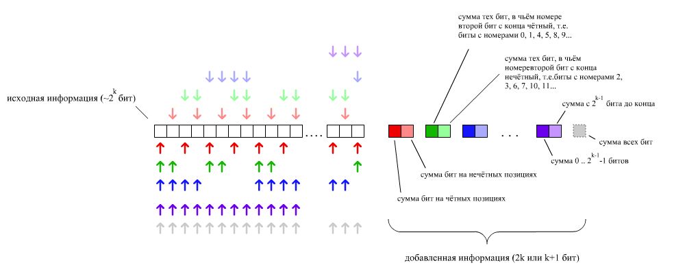
Соответствие добавленной информации исходным битам. Первый вариант кодирования соответствует использованию битов, раскрашенных в тёмные и светлые цвета, оптимизация — в тёмные цвета и серый
Легко понять, что если в одном бите из строки допущена ошибка, то с помощью дописанных пар бит можно точно определить, какой именно бит ошибочный. Это объясняется тем, что каждая пара определяет один бит номера ошибочного бита в строке. Всего пар , следовательно мы имеем бит номера ошибочного бита, что вполне достаточно: общее число бит строки не превосходит .
Теперь заметим, что в случае наличия ошибки в исходной строке, ровно один бит в каждой паре будет равен единице. Тогда можно оставить только один бит из пары. Однако этого будет недостаточно, поскольку если только один добавленный бит не соответствует строке, то нельзя понять, ошибка в нём или в строке. На этот случай можно добавить ещё один контрольный бит — всех битов строки.
Итого, увеличивая код длиной на , можно обнаружить и исправить одну ошибку.
См. также
- Обнаружение и исправление ошибок кодирования
Источники информации
- Wikipedia — Hamming code
