Unknown flow rate hysys как исправить

#1

#2

Liza Admani

#3

processengbd

#4

jewel10

#5

Nazia

#6

Freelance Process Engineer

#7

Neelakantan

#8

RockDock

#9

Bobby Strain

#10

Nazia

#11

jewel10

#12

Neelakantan

#13

Freelance Process Engineer

#14

jewel10

#15

Nazia

#16

Freelance Process Engineer

#17

Freelance Process Engineer

#18

Nazia

#19

Neelakantan

#20

Nazia

Start HYSYS then choose “File, New, Case”. On this screen which opens, which is called the “Basis Environment”, the “Components” tab at the bottom and the default radio button “HYSYS Databanks” should be selected. Next, click “Add” to add components from the database to your project.

After selecting “Add”, the screen above opens where you can add components to the project. HYSYS has a wide range of build-in components, but you must specify which components you will be using. In this case, we are going to use the C 1 – C 5 paraffins, so we begin choosing them and using the “Add Pure” button”.

After highlighting the component you want, click the “Add Pure” button”. Repeat to add all the C 1 – C 5 normal paraffins. You can use the default name “Component List-1”. If you make a mistake, use the “Delete” button to remove the component. When you are done, close the box using the “x” in the upper right corner. You don’t need to save anything at this point.

When the “Simulation Basis Manager” window comes back, chose the “Fluid Pkgs” tab along the bottom to open the screen above. This is where you will tell HYSYS what thermodynamics simulator you want to use. Click on the “Add” button.

In the “Fluid Package: Basis -1” window (above), check that the “HYSYS” and “All Types” radio buttons are selected, then scroll down the “Property Package Selection” window at the left and choose “UNIQUAC”. You can choose other models, but choose wisely, not indiscriminately. When finished, close the “Fluid Package” window using the “x” in the top right corner.

This returns us to the “Simulation Basis Manager” and completes the minimum required operations in the basis environment. Now, click on the button in the lower right corner: “Enter Simulation Environment”. The simulation environment is where the process is built. Transitioning to the simulation environment, you may see some warnings. Choose “OK” to take default values.

Next, click on the blue arrow near the top on the “Case (Main)” tool window (which has the equipment icons), then move over to the “PFD – Case (Main)” window, which is where the process flow diagram (PFD) will be built, and click somewhere on the window. The arrow, representing a process stream, will appear on the PFD window.

The arrow is labeled “ 1” by default and is a flow stream. In many instances, HYSYS will calculate properties of streams, but we also have the ability to specify properties. Always be cognizant of the fact that the phase rule limits the number of properties you can specify. In this case, we are beginning with an inlet stream to the PFD, and we want to tell HYSYS what the properties are. To do this, begin by double-clicking on the stream (the arrow). A new window will open.

We are going to specify the composition of this feedstream. With a specified composition, if the mixture is a single phase, we can also choose T and P to completely specify thermodynamic properties. If it forms two phases, we can only specify T or P, not both. We will see how HYSYS handles this shortly. Click on “Composition” in the left window first.

We can enter the composition of the stream many ways. HYSYS allows weight or mole fraction and other systems. Note that all the components you specified in the basis environment are in the table to the right. Below the table, find the “Edit” button and click on it to open a new window.

In this screen, we can choose the composition basis, but we want to stick with mole fractions. Highlight the methane mole fraction, and type “ 1” and press <enter>. The highlight moves to the Ethane row, then type “ 2”, followed on the next row by “ 3”, then “ 4” then “ 5”. You have specified 1 part methane, 2 parts ethane, 3 parts propane, etc. Next, click on “Normalize” over on the right-hand side to make these relative amounts into mole fractions. The screen then updates.

Your composition should look as given above. The “normalize” button makes the mole fractions add to 1 and saves you the trouble. Now click OK, and this screen for inputting composition will close.

Notice now that the message in yellow is “Unknown Temperature”. HYSYS will keep informing you where it doesn’t have enough information. Click on the “Conditions” link over on the left-hand side of the worksheet, and we will see how to specify conditions.

Highlight the box to the right of “Temperature (C)” and enter “ 200”. Note that as you type, a box to the right opens and displays the units “C”. When you press <enter>, you accept these default units. Alternatively, you could click on the dropdown arrow, and choose new units, but let’s practice that process with pressure rather than temperature, so just accept the default units.

Note that the message now says “Unknown Pressure”. Highlight the input box for pressure, type “ 1”, then click on the pressure unit dropdown menu and choose “atm”. When you press <enter>, the pressure (1 atm) is converted to 101. 3 k. Pa and that will appear in the pressure box. Alternately, you could have entered “ 101. 3” and taken the default units. The yellow message bar should now say “Unknown Flowrate”. Enter “ 1” in the “Molar Flow (kgmole/hr)” input box.

Once you have entered T, P, and a flowrate, the message bar should change to green and say “OK”. HYSYS computes all the remaining conditions. Note that the conditions you specified are in blue, those HYSYS computed are in black. Note especially the box “Vapour/Phase Fraction” which is computed to be 1. 0000. This means the stream is all vapor, and in this case, the stream is actually superheated.

Now, highlight the temperature input box and press the delete key. Let’s do a dewpoint calculation. Highlight the “Vapour/Phase Fraction” input box, and enter “ 1”. You have now specified the pressure and by specifying the vapor fraction to be 1, you are specifying two phases by telling HYSYS you want the dewpoint and that satisfies the phase rule. The two phases are a vapor phase and an infinitely small droplet of liquid phase.

You should have the conditions given above. Note that the dewpoint is 11. 59ºC at 101. 3 k. Pa. Note also that you are unable to highlight the temperature input box anymore, and the text in the box is now black. This is because temperature is a computed result. Now, how would you find the composition of the infinitely small liquid droplet in equilibrium with the vapor phase? Click on the “Composition” link in the left-hand box.

You will see the window where you originally entered the composition, and the composition you entered was the overall composition. Find the scroll bar below the list of components and scroll to the right. As you scroll, you will see the vapor phase composition to be identical to the overall composition (it is all vapor after all) and as you get all the way to the right, you will see the column titled ”Liquid Phase”. This is the composition of the infinitely small droplet of liquid.

Now, go back to the “Conditions” link, and enter “ 0” in the vapor fraction input box. You are now specifying a bubble-point calculation. You will have an infinitely small bubble of vapor in the liquid. Note that the bubble-point is -231. 2ºC – quite cold because methane is very volatile.

Go back to the “Composition” link, and check the vapor composition. It is 100% methane because of the very high relative volatility of methane at this temperature. If you want to see the K values, click on the “K Value” link in the left column and you will see that the methane K value is 15. 00 while all the other components have K values smaller than 10 -20.

Finally, enter “ 0. 5” for the vapor phase fraction on the “Conditions” link.

Check the “Composition” link to see the vapor and liquid compositions. You may need to expand the width of the window to see both the vapor and liquid compositions at the same time.

Similar calculations can be done fixing temperature, and computing dew-pressure and bubble-pressure. To do this, delete the pressure, and enter a fixed temperature – say 50ºC, then put in a vapor faction of 1, 0, and 0. 5 in succession. The screen capture above shows a dew-pressure of 378. 8 k. Pa at 50ºC. An infinitesimally small droplet of liquid would be formed when a gaseous mixture at 50ºC is compressed at constant T to 378. 8 k. Pa.

For a vapor faction of 0 at 50ºC, an infinitesimally small bubble of vapor would be formed when a liquid mixture at 50ºC is at 2497 k. Pa. Check the vapor composition and you will see it is 53. 4726% methane.

Practice Exercises • Find the pressure and vapor and liquid composition at T=50ºC, vapor fraction = 0. 5 • Repeat the calculations in this tutorial, but use the Peng. Robinson equation of state instead of UNIQUAC. To change to Peng-Robinson: – Go back to the basis environment by clicking on the beaker icon on the toolbar or choosing Simulation/Enter Basis Environment from the menu. – Click the Fluid Pkgs tab, highlight Basis 1 – UNIQUAC line, click “view”, choose Peng-Robinson from the Property Package Selection list. – Close window and click “Return to Simulation Environment”. • Compare results of Peng-Robinson to UNIQUAC. Why are the results different but approximately the same?

INTELLIGENT WORK FORUMS
FOR ENGINEERING PROFESSIONALS

Log In

В специализированном окне колонны перейдите на страницу Монитор закладки Данные. В групповой рамке Спецификации перечислены спецификации, принятые программой по умолчанию. Вы можете использовать эти спецификации или заменить их другими, более подходящими для Вашей задачи. Число и тип спецификаций зависит от выбранного Вами типа колонны.

Спецификация может иметь один из следующих статусов – активная, оценка или текущая. Активными являются спецификации, значения которых должны быть достигнуты в результате расчета колонны.

Для абсорбера с ребойлером активной спецификацией по умолчанию является отбор пара сверху колонны. Рассчитаем колонну на другую спецификацию – мольная доля метана в кубовой жидкости составляет 0.01. Нажмите кнопку Добавить спецификацию, выберите тип спецификации – Доля компонента и задайте следующие параметры спецификации:

Укажите, что новая спецификация является активной (поставьте флажок в столбце Активн.), а прежняя спецификация – Отбор пара сверху не является активной (уберите флажок). Обратите внимание, что при этом меняется значение в поле Число степеней свободы. Когда Вы делаете спецификацию активной, число степеней свободы уменьшается на одну. Соответственно, когда Вы делаете спецификацию неактивной, число степеней свободы увеличивается на одну. Расчет колонны можно начинать, когда число степеней свободы равно нулю.

Запустите колонну на счет – кнопка Пуск. Когда расчет колонны будет завершен, Вы можете просмотреть результаты на закладках Рабочая таблица и Результаты.

2.12 Использование встроенных электронных таблиц

Проведем исследование, как зависит выход этана от выходного давления детандера. Воспользуемся для этого операцией Электронная таблица.

Операция Электронная таблица позволяет использовать вычислительные возможности электронных таблиц для проведения расчетов в технологической схеме. Операция осуществляет доступ практически ко всем переменным схемы. Поля таблицы обновляются всякий раз, когда меняются переменные технологической схемы. Электронная таблица HYSYS использует стандартные приемы работы со строками и столбцами. В любое поле можно импортировать переменную, или задать число или формулу.

Добавьте операцию Электронная таблица. Перейдите на закладку Электронная таблица. Сначала следует настроить электронную таблицу так, чтобы в ней отражалась нужная нам информация. Текстовые поля добавляются путем простого ввода их с клавиатуры, а для добавления переменной из технологической схемы нажмите правую кнопку мыши и выберите команду Импорт переменной.

Задайте следующие параметры:

Теперь Вы можете менять давление после детандера, просто задавая новое значение в ячейке В1. При этом схема будет пересчитана, значения в электронной таблице обновятся, и в ячейке В6 Вы увидите новое значение извлечения этана.

2.13 Проведение расчетного исследования

Давайте проведем несколько расчетов, в которых будем менять давление потока 5 от 15 до 30 бар и следить за извлечением этана (ячейка В6 в электронной таблице). HYSYS позволяет сделать это автоматически, используя процедуру Расчетное исследование из Книги данных.

С помощью этого инструмента можно проводить расчетные исследования задачи. Для этого следует определить независимые и зависимые переменные. Для каждой независимой переменной задаются нижняя и верхняя граница и интервал ее изменения. Программа изменяет независимую переменную в соответствии с заданной настройкой, пересчитывает полностью схему и запоминает значения зависимых переменных. Затем снова изменяет независимую переменную и т.д. Получается некоторый набор точек, отражающий зависимость переменных схемы от заданных независимых (варьируемых) переменных. Результаты расчетного исследования можно получить в графическом или табличном виде.

Откройте Книгу данных(Ctrl-D) на закладке Переменные и выберите переменные, указанные в таблице.

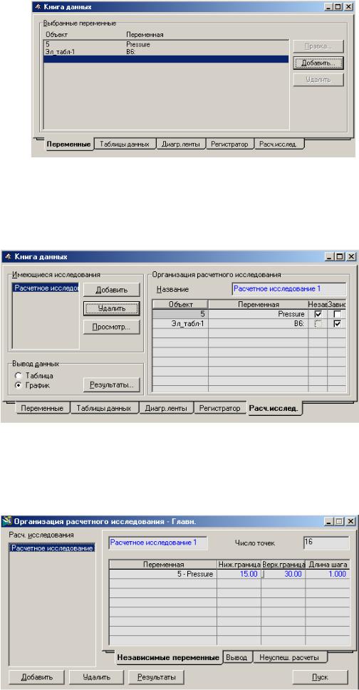
Перейдите на закладку Расчетные исследования. С помощью кнопки Добавить организуйте Исследование 1. С помощью флажков укажите, что давление в потоке 5 является независимой переменной, а извлечение этана (ячейка В6) – зависимой.

Для того, чтобы провести исследование, необходимо задать интервал изменения независимой переменной. Нажмите кнопку Просмотр, и Вы попадете в окно Организация расчетного исследования, в котором задайте следующие величины:

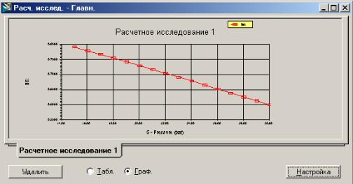
Чтобы начать расчет, нажмите кнопку Пуск. Результаты выводятся на экран с помощью кнопки Результаты. Обратите внимание, что эти результаты можно выводить как в виде таблицы, так и в виде графика.

3 Содержание промежуточных отчётов и отчёта по курсовому проекту

Отчёт должен быть выполнен в среде Office Word и содержать следующие разделы:

–вводную информацию по моделируемому процессу 1-3 стр.;

–порядок выполнения работы в программе HYSYS;

–таблица с вводимыми переменными (пример таблицы 1,2,3);

–таблица с размерами аппаратов (пример таблица 4)

–общую расчётную схему (пример рисунок 1);

–таблицы, формированные программой HYSYS, с данными по всем потокам и аппаратам.

(для вывода на печать информации о потоке или аппарате необходимо войти в него на схеме двойным нажатием мыши, после чего выбрать в меню HYSYS вкладку файл, далее печать и подтверждение печати в отдельном окне)

Таблица 1 – Переменные введённые оператором (аппаратура)

Таблица 2 – Переменные введённые оператором (потоки материальные)

Таблица 3 – Переменные введённые оператором (потоки энергетические)

Таблица 4 – Основные размеры аппаратов

4 Задания для выполнения

Задание № 1 Провести подготовку газа к нефтепереработке (параметры исходного

газа указаны в таблице №1) методом последовательного компремирования и сепарирования (общие требования к технологии указаны в таблице 1). Подготовленный газ должен соответствовать требованиям по содержанию заданного компонента (требования по заданному компоненту и его содержанию указаны в таблице 1) при этом его извлечение должно быть максимальным из других потоков. В процессе компремирования температура на выходе из любого компрессора не должна превышать 147 °С. Чисто последовательных ступеней компрессора, сепараторов и холодильников не ограничивается, но должно быть минимально возможным для достижения требуемых качественных параметров. Отчёт предоставить в соответствии с методическими указаниями.

Таблица 5 – Исходные данные для проектирования установки выделения газа

Recommended :
– Tips on Succession in FREE Subscription
– Subscribe FREE – Processing & Control News

“I was doing Depressuing using HYSYS and flare network back pressure calculation using FLARENET for conventional Blowdown valves with restriction (BDV/RO). Peak flow of Depressuring unit in HYSYS which obtained from initial depressuring and based on initial depressuring pressure to Atmospheric pressure, is used as input to FLARENET.

Above was a question raised by an engineer who was conducting plant blowdown and flare network studies.

First far most important thing is that there will be total plant or segregated zone blowdown. This type of blowdown will results simultaneous opening of all BDVs within a zone and simultaneous blowdown of multiple sections. One shall not consider SINGLE BDV opening ONLY. Simultaneous blowdown will results high total blowdown rate and induced high back pressure to each BDV / RO within the blowdown zone.

In many events, the flow passing the RO is CRITICAL flow where the back pressure from flare network is lower than the fluid critical pressure (Pc). Read more in “A refresh to Process Engineer on few phenomenons in restriction orifice”. Under critical flow condition, the back pressure has no impact to the flow rate passing through the RO (assume backpressure does not affect the vena contracta cross sectional area). Thus, peak flow calculated in HYSYS depressuring unit considering backpressure of ATM is still remain same if the backpressure (Pb) is lower than critical pressure (Pc).

However, for many rare cases when the system pressure is low, hence the critical is much lower. This potentially results back pressure high than critical pressure and cause SUBCRITICAL flow condition. Under this condition, backpressure has impact to the peak flow calculated by HYSYS.

Knowing back pressure may affect peak flow under subscritical flow condition, some level of checking and iteration may required.

Iteration as proposed above could be very time consuming and not all the BDV/RO required iterate update. Infact only those BDV/RO experiencing Subcritical flow would need to involve in the iteration process.

The following steps may be considered :

i) For initial step, use ATM in HYSYS for depressuring to estimate the peak flow
ii) Peak flow estimated in HYSYS will be entered into FLARENET to calculate back pressure at each BDV/ROs.
iii) Compare each BDV/RO Critical pressure (Pc) and Back pressure (Pb). If Pc is higher than Pb, that particular BDV/RO need not involve in the iteration.
iv) Identify those BDV/RO with Pc less than Pb. Re-adjust back pressure in HYSYS base on calculated Pb from FLARENET to obtain a new peak flow.
v) Reenter and rerun in FLARENET.
vi) Repeat step (iii) to (v) till backpressure in HYSYS and FLARENET are matched.

Above will significantly reduce the iteration time.

Related Topic

• Don’t misunderstood depressuring
• Depressuring within 15 minutes no longer applicable ?
• Bug in ASPENTECH HYSYS 2006 Dynamic Depressuring Fisher Valve model
• Controlled and Non-controlled Type Depressuring
• How to apply valve equation in HYSYS Depressuring ?
• How to determine if a restriction orifice will experience cavitation ?